Open Journal of Discrete Applied Mathematics
ISSN: 2617-9687 (Online) 2617-9679 (Print)
DOI: 10.30538/psrp-odam2019.0014
Some properties of the solutions of the difference equation \(x_{n+1}=a x_{n}+\dfrac{b x_{n} x_{n-4}}{c x_{n-3}+dx_{n-4}}\)
Mathematics Department, Faculty of Science, King Abdulaziz University, P. O. Box 80203, Jeddah 21589, Saudi Arabia.; (A.S & E.M.E)
General studies department, Jeddah College of Telecom and Electronics, TVTC, B.P. 2816, Jeddah 21461, Saudi Arabia.; (A.S)
Department of Mathematics, Faculty of Science, Mansoura University, Mansoura 35516, Egypt.; (E.M.E)
\(^{1}\)Corresponding Author: sanbo@cte.edu.sa
Abstract
Keywords:
1. Introduction
Our aim in this paper is to investigate the behavior of the solution of the following nonlinear difference equation
Recently there has been a great interest in studying the qualitative properties of rational difference equations. Some prototypes for the development of the basic theory of the global behavior of nonlinear difference equations of order greater than one come from the results for rational difference equations [1, 2, 3, 4, 5, 6, 7, 8, 9, 10, 11, 12, 13, 14, 15].
However, there have not been any effective general methods to deal with the global behavior of rational difference equations of order greater than one so far. From the known work, one can see that it is extremely difficult to understand thoroughly the global behaviors of solutions of rational difference equations although they have simple forms (or expressions). One can refer to [16, 17, 18, 19, 20, 21, 2, 23, 24, 25, 26, 27, 28, 29, 30, 31, 32, 33, 34, 35, 36, 37, 38, 39, 40, 41, 42, 43, 44, 45, 46, 47] for examples to illustrate this. Therefore, the study of rational difference equations of order greater than one is worth further consideration.
Many researchers have investigated the behavior of the solution of difference equations, for example,
Elsayed et al. [37] has obtained results concerning the dynamics and global attractivity of the rational difference equation \begin{equation*} x_{n+1}=\dfrac{ax_nx_{n-2}}{bx_{n-2}+cx_{n-3}}. \end{equation*} Aloqeili [18] has obtained the solutions of the difference equation \begin{equation*} x_{n+1}=\dfrac{x_{n-1}}{a-x_{n}x_{n-1}}. \end{equation*} Simsek et al. [43] obtained the solution of the difference equation \begin{equation*} x_{n+1}=\dfrac{x_{n-3}}{1+ x_{n-1}} \end{equation*} Cinar [22, 23, 24] got the solutions of the following difference equations \begin{equation*} x_{n+1}=\dfrac{x_{n-1}}{1+ax_{n}x_{n-1}}, x_{n+1}=\dfrac{x_{n-1}}{ -1+ax_{n}x_{n-1}}, x_{n+1}=\dfrac{ax_{n-1}}{1+bx_{n}x_{n-1}}. \end{equation*} In [48], Ibrahim got the form of the solution of the rational difference equation \begin{equation*} x_{n+1}=\dfrac{x_nx_{n-2}}{x_{n-1}(a+bx_{n}x_{n-2})}. \end{equation*} Karatas et al. [46] got the solution of the difference equation \begin{equation*} x_{n+1}=\dfrac{x_{n-5}}{1+x_{n-2}x_{n-5}}. \end{equation*} Here, we recall some notations and results which will be useful in our investigation. Let \(I\) be some interval of real numbers and let \begin{equation*} f : I^{k+1} \rightarrow I, \end{equation*} be a continuously differentiable function. Then for every set of initial conditions \(x_{-k}, x_{-k+1}, x_{-k+2}, ..., x_{0} \in I\), the difference equationDefinition 1. A point \(\bar x \in I\) is called an \textit{equilibrium point} of Equation (2) if \(\bar x=f(\bar x,\bar x,...,\bar x)\). That is, \(x_n = \bar x\) for \(n \geq 0\), is a solution of Equation (2), or equivalently, \(\bar x\) is a fixed point of \(f\).
Definition 2.
- The equilibrium point \(\bar x\) of Equation (2) is locally stable if for every \(\varepsilon> 0\), there exists \(\delta > 0\) such that for all \(x_{-k}, x_{-k+1}, x_{-k+2}, ..., x_{0} \in I,\) with \begin{equation*} |x_{-k}-\bar x|+|x_{-k+1}-\bar x|+|x_{-k+2}-\bar x|+...+|x_{0}-\bar x| < \delta, \end{equation*} we have \(|x_n - \bar x| < \varepsilon\), for all \(n \geq -k\).
- The equilibrium point \(\bar x\) of Equation (2) is locally asymptotically stable if \(\bar x\) is locally stable solution of Equation (2) and there exists \( \gamma > 0\), such that for all \(x_{-k}, x_{-k+1}, x_{-k+2}, ..., x_{0} \in I, \) with \begin{equation*} |x_{-k}-\bar x|+|x_{-k+1}-\bar x|+|x_{-k+2}-\bar x|+...+|x_{0}-\bar x| < \delta, \end{equation*} we have \(\displaystyle \lim_{n\rightarrow \infty} x_n = \bar x\).
- The equilibrium point \(\bar x\) of Equation (2) is global attractor if for all \(x_{-k}, x_{-k+1}, ... , x_{0} \in I\) we have \begin{equation*} \lim_{n\rightarrow \infty} x_n = \bar x. \end{equation*}
- The equilibrium point \(\bar x\) of Equation (2) is globally asymptotically stable if \(\bar x\) is locally stable, and \(\bar x\) is also a global attractor of Equation (2).
- The equilibrium point \(\bar x\) of Equation (2) is unstable if \(\bar x\) is not locally stable.
Theorem 3. Assume that \(p, q \in \mathbb{R}\) and \(k \in \{0, 1, 2, ...\}\). Then \(|p| + |q| < 1\) is a sufficient condition for the asymptotic stability of the difference equation \begin{equation*} x_{n+1} + px_n + qx_{n-k} = 0, n = 0, 1, \ldots \end{equation*}
Remark 1. The theorem can be easily extended to a general linear equations of the form
Theorem 4. Let \([a, b]\) be an interval of real numbers and assume that \begin{equation*} g:[a, b]^3\rightarrow [a, b], \end{equation*} is a continuous function satisfying the following properties:
- \(g(x,y,z)\) is nondecreasing in \(x\) and \(z\) in \([a, b]\) for each \(y \in[a, b]\), and is nonincreasing in \(y\in[a, b]\) for each \(x\) and \(z\) in \( [a, b]\)
- if \((m,M)\in [a, b]\times [a, b]\) is a solution of the system \begin{equation*} M=g(M,m,M),\qquad m=g(m,M,m), \end{equation*} then \(m=M\).
2. Local stability of equation (1)
In this section we investigate the local stability character of the solutions of Equation (1). Equation (1) has a unique equilibrium point and is given by \begin{equation*} \bar x=a \bar x+\dfrac{b \bar x^2}{ c \bar x+d \bar x}, \end{equation*} or \begin{equation*} \bar x^2(1-a)(c+d)=b \bar x^2, \end{equation*} then if \((1-a)(c+d)\not=b\) , then the unique equilibrium point is \(\bar x=0\).\\ Define the following function \begin{equation*} \begin{array}{llll} f:(0,\infty)^3\rightarrow (0,\infty) & & & \\ f(u,v,w)=a u+\dfrac{b u w}{c v+d w}. & & & \end{array} \end{equation*} It follows that \begin{equation*} f_u(u,v,w)=a +\dfrac{b w}{c v+d w}, \quad f_v(u,v,w)=-\dfrac{bc u w}{(c v+d w)^2},\quad f_w(u,v,w)=\dfrac{b cu v}{(c v+d w)^2}. \end{equation*} Then \begin{equation*} f_u(\bar x,\bar x, \bar x)=a +\dfrac{b }{c +d}, \quad f_v(\bar x,\bar x, \bar x)=-\dfrac{bc}{(c +d )^2},\quad f_w(\bar x,\bar x, \bar x)=\dfrac{bc}{ (c +d )^2}. \end{equation*} The linearized equation of Equation (1) about \(\bar x\) isTheorem 5. Assume that \begin{equation*} b(d+3c)< (1-a)(c+d)^2. \end{equation*} Then the equilibrium point of Equation (1) is locally asymptotically stable.
Proof. It follows from Theorem 3 that Equation (5) is asymptotically stable if \begin{equation*} \left|a +\dfrac{b }{c +d}\right|+\left|\dfrac{bc}{(c +d )^2}\right|+\left| \dfrac{bc}{(c +d )^2}\right|< 1, \end{equation*} or \begin{equation*} a +\dfrac{b }{c +d}+\dfrac{2bc}{(c +d )^2}< 1, \end{equation*} and so, \begin{equation*} \dfrac{b(d+3c) }{(c +d )^2}< (1-a). \end{equation*} The proof is complete.
3. Global attractor of the equilibrium point of equation (1)
In this section we investigate the global attractivity character of solutions of Equation (1).Theorem 6. The equilibrium point \(\bar x\) of Equation (1) is global attractor if \(d(1-a)\not=b\)
Proof. Let \(p,q\) be real numbers and assume that \(g:[p, q]^3\rightarrow [p, q]\) is a function defined by \( g(u,v,w)=au+\dfrac{buw}{cv +dw}\), then we can easily see that the function \( g(u,v,w)\) is increasing in \(u,w\) and decreasing in \(v\). Suppose that \((m,M)\) is a solution of the system \begin{equation*} M=g(M,m,M),\qquad m=g(m,M,m). \end{equation*} Then from Equation (1), we see that \begin{equation*} M=aM+\dfrac{bM^2}{cm +dM},\qquad m=am+\dfrac{bm^2}{cM +dm} \end{equation*} or \begin{equation*} M(1-a)=\dfrac{bM^2}{cm +dM},\qquad m(1-a)=\dfrac{bm^2}{cM +dm} \end{equation*} then \begin{equation*} c(1-a)mM+d(1-a)M^2=bM^2,\qquad c(1-a)mM+d(1-a)m^2=bm^2 \end{equation*} subtracting, we obtain \begin{equation*} d(1-a)(M^2-m^2)=b(M^2-m^2). \end{equation*} Since \(d(1-a)\not=b\) therefore \begin{equation*} M=m. \end{equation*} It follows from Theorem 4 that \(\bar x\) is a global attractor of Equation (1), and then the proof is complete.
4. Boundedness of solutions of equation (1)
In this section we study the boundedness of solutions of Equation (1).Theorem 7. Every solution of Equation (1) is bounded if \(a+\dfrac{b}{d}< 1\).
Proof. Let \(\{x_n\}_{n=-4}^\infty\) be a solution of Equation (1). It follows from Equation (1) that \begin{equation*} x_{n+1}=a x_{n}+\dfrac{b x_{n} x_{n-4}}{c x_{n-3}+dx_{n-4}}\leq a x_{n}+ \dfrac{b x_{n} x_{n-4}}{dx_{n-4}}=\left(a+\dfrac{b}{d}\right)x_{n}. \end{equation*} Then \(x_{n+1}\leq x_{n}, \quad \forall n\geq 0\). Then the sequence \( \{x_n\}_{n=-4}^\infty\) is decreasing and so is bounded from above by \( M=\max\{x_{-4}, x_{-3}, x_{-2}, x_{-1}, x_0\}\).
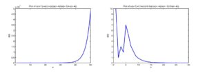
For explaining the results of this section, we consider numerical example for \(x_{-4}=10, x_{-3}=1, x_{-2}=3, x_{-1}=2, x_0=7\). (See Figure 1). \begin{center}Figure 1. Left \(a=1, b=1, c=1, d=1\) which don’t satisfy the boundedness conditions (the solution is unbounded). Right \(a=0.5, b=0.5, c=1, d=2\) which satisfy the boundedness conditions (the solution is bounded).
5. Special cases of equation (1)
Our goal in this section is to find a specific form of the solutions of some special cases of Equation (1) when , \(a,b,c\) and \(d\) are integers and give numerical examples of each case.5.1. First case: on the difference equation \(x_{n+1}= x_{n}+\dfrac{x_{n} x_{n-4}}{ x_{n-3}+x_{n-4}}\)
In this subsection we study the following special case of Equation (1):Theorem 8. Let \(\{x_n\}_{n=-4}^\infty\) be a solution of Equation (6). Then for \(n=0,1,2,...\) \begin{equation*} \left\{ \begin{array}{llll} \displaystyle x_{4n}=r\prod_{i=1}^{n}\dfrac{(A_if+2B_ie)}{(B_if+A_ie)} \dfrac{(A_ig+2B_if)}{(B_ig+A_if)}\dfrac{(A_ih+2B_ig)}{(B_ih+A_ig)} \dfrac{ (A_ir+2B_ih)}{(B_ir+A_ih)} , & & & \\ \displaystyle x_{4n+1}=r\prod_{i=1}^{n+1}\dfrac{(A_if+2B_ie)}{(B_if+A_ie)} \prod_{i=1}^{n}\dfrac{(A_ig+2B_if)}{(B_ig+A_if)}\dfrac{(A_ih+2B_ig)}{ (B_ih+A_ig)}\dfrac{(A_ir+2B_ih)}{(B_ir+A_ih)}, & & & \\ \displaystyle x_{4n+2}=r\prod_{i=1}^{n+1}\dfrac{(A_if+2B_ie)}{(B_if+A_ie)} \dfrac{(A_ig+2B_if)}{(B_ig+A_if)} \prod_{i=1}^{n}\dfrac{(A_ih+2B_ig)}{ (B_ih+A_ig)}\dfrac{(A_ir+2B_ih)}{(B_ir+A_ih)}, & & & \\ \displaystyle x_{4n+3}=r\prod_{i=1}^{n+1}\dfrac{(A_if+2B_ie)}{(B_if+A_ie)} \dfrac{(A_ig+2B_if)}{(B_ig+A_if)}\dfrac{(A_ih+2B_ig)}{(B_ih+A_ig)} \prod_{i=1}^{n}\dfrac{(A_ir+2B_ih)}{(B_ir+A_ih)} , & & & \end{array} \right. \end{equation*} where \(x_{-4}=e, x_{-3}=f, x_{-2}=g, x_{-1}=h, x_0=r\), \(\{A_m\}_{m=1}^ \infty=\{1,3,7,17,41,...\}\), \(\{B_m\}_{m=1}^\infty=\{1,2,5,12,29,...\}\) \( A_m=2A_{m-1}+A_{m-2}, B_m=2B_{m-1}+B_{m-2}, m\geq 1, A_{-1}=-1\), \(A_0=1\), \( B_{-1}=1, B_0=0\), or also \(A_m=2B_{m-1}+A_{m-1}, B_m=B_{m-1}+A_{m-1}, m\geq 0 \), and \(\displaystyle \prod_{i=1}^{0}G_i=1\).
Proof. For \(n=0\), the result holds. Now suppose that our assumption holds for \(n-1\) and for \(n-2\). That is \begin{equation*} \left\{ \begin{array}{llll} \displaystyle x_{4n-8}=r\prod_{i=1}^{n-2}\dfrac{(A_if+2B_ie)}{(B_if+A_ie)} \dfrac{(A_ig+2B_if)}{(B_ig+A_if)}\dfrac{(A_ih+2B_ig)}{(B_ih+A_ig)} \dfrac{ (A_ir+2B_ih)}{(B_ir+A_ih)} , & & & \\ \displaystyle x_{4n-7}=r\prod_{i=1}^{n-1}\dfrac{(A_if+2B_ie)}{(B_if+A_ie)} \prod_{i=1}^{n-2}\dfrac{(A_ig+2B_if)}{(B_ig+A_if)}\dfrac{(A_ih+2B_ig)}{ (B_ih+A_ig)}\dfrac{(A_ir+2B_ih)}{(B_ir+A_ih)}, & & & \\ \displaystyle x_{4n-6}=r\prod_{i=1}^{n-1}\dfrac{(A_if+2B_ie)}{(B_if+A_ie)} \dfrac{(A_ig+2B_if)}{(B_ig+A_if)} \prod_{i=1}^{n-2}\dfrac{(A_ih+2B_ig)}{ (B_ih+A_ig)}\dfrac{(A_ir+2B_ih)}{(B_ir+A_ih)}, & & & \\ \displaystyle x_{4n-5}=r\prod_{i=1}^{n-1}\dfrac{(A_if+2B_ie)}{(B_if+A_ie)} \dfrac{(A_ig+2B_if)}{(B_ig+A_if)}\dfrac{(A_ih+2B_ig)}{(B_ih+A_ig)} \prod_{i=1}^{n-2}\dfrac{(A_ir+2B_ih)}{(B_ir+A_ih)}, & & & \end{array} \right. \end{equation*} \begin{equation*} \left\{ \begin{array}{llll} \displaystyle x_{4n-4}=r\prod_{i=1}^{n-1}\dfrac{(A_if+2B_ie)}{(B_if+A_ie)} \dfrac{(A_ig+2B_if)}{(B_ig+A_if)}\dfrac{(A_ih+2B_ig)}{(B_ih+A_ig)} \dfrac{ (A_ir+2B_ih)}{(B_ir+A_ih)} , & & & \\ \displaystyle x_{4n-3}=r\prod_{i=1}^{n}\dfrac{(A_if+2B_ie)}{(B_if+A_ie)} \prod_{i=1}^{n-1}\dfrac{(A_ig+2B_if)}{(B_ig+A_if)}\dfrac{(A_ih+2B_ig)}{ (B_ih+A_ig)}\dfrac{(A_ir+2B_ih)}{(B_ir+A_ih)}, & & & \\ \displaystyle x_{4n-2}=r\prod_{i=1}^{n}\dfrac{(A_if+2B_ie)}{(B_if+A_ie)} \dfrac{(A_ig+2B_if)}{(B_ig+A_if)} \prod_{i=1}^{n-1}\dfrac{(A_ih+2B_ig)}{ (B_ih+A_ig)}\dfrac{(A_ir+2B_ih)}{(B_ir+A_ih)}, & & & \\ \displaystyle x_{4n-1}=r\prod_{i=1}^{n}\dfrac{(A_if+2B_ie)}{(B_if+A_ie)} \dfrac{(A_ig+2B_if)}{(B_ig+A_if)}\dfrac{(A_ih+2B_ig)}{(B_ih+A_ig)} \prod_{i=1}^{n-1}\dfrac{(A_ir+2B_ih)}{(B_ir+A_ih)}. & & & \end{array} \right. \end{equation*} Now it follows from Equation (6) that \begin{equation*} \begin{array}{llll} \displaystyle x_{4n} = \displaystyle x_{4n-1}+\dfrac{ x_{4n-1} x_{4n-5}}{ x_{4n-4}+x_{4n-5}}= r\prod_{i=1}^{n}\dfrac{(A_if+2B_ie)}{(B_if+A_ie)}\dfrac{ (A_ig+2B_if)}{(B_ig+A_if)}\dfrac{(A_ih+2B_ig)}{(B_ih+A_ig)} \prod_{i=1}^{n-1} \dfrac{(A_ir+2B_ih)}{(B_ir+A_ih)} \Bigg(1+ & \\ \dfrac{\displaystyle r\prod_{i=1}^{n-1}\dfrac{(A_if+2B_ie)}{ (B_if+A_ie)}\dfrac{(A_ig+2B_if)}{(B_ig+A_if)}\dfrac{(A_ih+2B_ig)}{(B_ih+A_ig) } \prod_{i=1}^{n-2}\dfrac{(A_ir+2B_ih)}{(B_ir+A_ih)}}{\displaystyle r\prod_{i=1}^{n-1}\dfrac{(A_if+2B_ie)}{(B_if+A_ie)} \dfrac{(A_ig+2B_if)}{ (B_ig+A_if)}\dfrac{(A_ih+2B_ig)}{(B_ih+A_ig)} \dfrac{(A_ir+2B_ih)}{ (B_ir+A_ih)} +r\prod_{i=1}^{n-1}\dfrac{(A_if+2B_ie)}{(B_if+A_ie)}\dfrac{ (A_ig+2B_if)}{(B_ig+A_if)}\dfrac{(A_ih+2B_ig)}{(B_ih+A_ig)} \prod_{i=1}^{n-2} \dfrac{(A_ir+2B_ih)}{(B_ir+A_ih)}}\Bigg) & \\ = \displaystyle r\prod_{i=1}^{n}\dfrac{(A_if+2B_ie)}{(B_if+A_ie)}\dfrac{ (A_ig+2B_if)}{(B_ig+A_if)}\dfrac{(A_ih+2B_ig)}{(B_ih+A_ig)} \prod_{i=1}^{n-1} \dfrac{(A_ir+2B_ih)}{(B_ir+A_ih)}\left(1+ \dfrac{1}{\dfrac{ (A_{n-1}r+2B_{n-1}h)}{(B_{n-1}r+A_{n-1}h)} +1}\right) & \\ = \displaystyle r\prod_{i=1}^{n}\dfrac{(A_if+2B_ie)}{(B_if+A_ie)}\dfrac{ (A_ig+2B_if)}{(B_ig+A_if)}\dfrac{(A_ih+2B_ig)}{(B_ih+A_ig)} \prod_{i=1}^{n-1} \dfrac{(A_ir+2B_ih)}{(B_ir+A_ih)}\left(1+ \dfrac{B_{n-1}r+A_{n-1}h}{ (A_{n-1}+B_{n-1})r+(2B_{n-1}+A_{n-1})h} \right) & \\ = \displaystyle r\prod_{i=1}^{n}\dfrac{(A_if+2B_ie)}{(B_if+A_ie)}\dfrac{ (A_ig+2B_if)}{(B_ig+A_if)}\dfrac{(A_ih+2B_ig)}{(B_ih+A_ig)} \prod_{i=1}^{n-1} \dfrac{(A_ir+2B_ih)}{(B_ir+A_ih)}\; \dfrac{ (A_{n-1}+2B_{n-1})r+(2B_{n-1}+2A_{n-1})h}{ (A_{n-1}+B_{n-1})r+(2B_{n-1}+A_{n-1})h} & \\ = \displaystyle r\prod_{i=1}^{n}\dfrac{(A_if+2B_ie)}{(B_if+A_ie)}\dfrac{ (A_ig+2B_if)}{(B_ig+A_if)}\dfrac{(A_ih+2B_ig)}{(B_ih+A_ig)} \prod_{i=1}^{n-1} \dfrac{(A_ir+2B_ih)}{(B_ir+A_ih)}\; \dfrac{A_{n}r+2B_{n}h}{B_{n}r+A_{n}h} & \\ = \displaystyle r\prod_{i=1}^{n}\dfrac{(A_if+2B_ie)}{(B_if+A_ie)}\dfrac{ (A_ig+2B_if)}{(B_ig+A_if)}\dfrac{(A_ih+2B_ig)}{(B_ih+A_ig)} \dfrac{ (A_ir+2B_ih)}{(B_ir+A_ih)}. & \end{array} \end{equation*} Similarly, \begin{equation*} \begin{array}{llll} \displaystyle x_{4n+1} = \displaystyle x_{4n}+\dfrac{ x_{4n} x_{4n-4}}{ x_{4n-3}+x_{4n-4}}= r\prod_{i=1}^{n}\dfrac{(A_if+2B_ie)}{(B_if+A_ie)}\dfrac{ (A_ig+2B_if)}{(B_ig+A_if)}\dfrac{(A_ih+2B_ig)}{(B_ih+A_ig)} \dfrac{ (A_ir+2B_ih)}{(B_ir+A_ih)}\end{array} \end{equation*}} {\small \begin{equation*} \begin{array}{llll} \Bigg(1+ \\ \dfrac{\displaystyle r\prod_{i=1}^{n-1}\dfrac{(A_if+2B_ie)}{ (B_if+A_ie)}\dfrac{(A_ig+2B_if)}{(B_ig+A_if)}\dfrac{(A_ih+2B_ig)}{(B_ih+A_ig) } \dfrac{(A_ir+2B_ih)}{(B_ir+A_ih)}}{\displaystyle r\prod_{i=1}^{n}\dfrac{ (A_if+2B_ie)}{(B_if+A_ie)}\prod_{i=1}^{n-1} \dfrac{(A_ig+2B_if)}{(B_ig+A_if)} \dfrac{(A_ih+2B_ig)}{(B_ih+A_ig)} \dfrac{(A_ir+2B_ih)}{(B_ir+A_ih)} +r\prod_{i=1}^{n-1}\dfrac{(A_if+2B_ie)}{(B_if+A_ie)}\dfrac{(A_ig+2B_if)}{ (B_ig+A_if)}\dfrac{(A_ih+2B_ig)}{(B_ih+A_ig)} \dfrac{(A_ir+2B_ih)}{ (B_ir+A_ih)}}\Bigg) \\ \end{array} \end{equation*} \begin{equation*} \begin{array}{llll} = \displaystyle r\prod_{i=1}^{n}\dfrac{(A_if+2B_ie)}{(B_if+A_ie)}\dfrac{ (A_ig+2B_if)}{(B_ig+A_if)}\dfrac{(A_ih+2B_ig)}{(B_ih+A_ig)} \dfrac{ (A_ir+2B_ih)}{(B_ir+A_ih)}\left(1+ \dfrac{1}{\dfrac{(A_{n}r+2B_{n}h)}{ (B_{n}r+A_{n}h)} +1}\right) \\ = \displaystyle r\prod_{i=1}^{n}\dfrac{(A_if+2B_ie)}{(B_if+A_ie)}\dfrac{ (A_ig+2B_if)}{(B_ig+A_if)}\dfrac{(A_ih+2B_ig)}{(B_ih+A_ig)} \dfrac{ (A_ir+2B_ih)}{(B_ir+A_ih)}\left(1+ \dfrac{B_{n}r+A_{n}h}{ (A_{n}+B_{n-1})r+(2B_{n}+A_{n})h} \right) \\ = \displaystyle r\prod_{i=1}^{n}\dfrac{(A_if+2B_ie)}{(B_if+A_ie)}\dfrac{ (A_ig+2B_if)}{(B_ig+A_if)}\dfrac{(A_ih+2B_ig)}{(B_ih+A_ig)} \dfrac{ (A_ir+2B_ih)}{(B_ir+A_ih)}\; \dfrac{(A_{n}+2B_{n})r+(2B_{n}+2A_{n})h}{ (A_{n}+B_{n})r+(2B_{n}+A_{n})h} \\ = \displaystyle r\prod_{i=1}^{n}\dfrac{(A_if+2B_ie)}{(B_if+A_ie)}\dfrac{ (A_ig+2B_if)}{(B_ig+A_if)}\dfrac{(A_ih+2B_ig)}{(B_ih+A_ig)} \dfrac{ (A_ir+2B_ih)}{(B_ir+A_ih)}\; \dfrac{A_{n+1}r+2B_{n+1}h}{B_{n+1}r+A_{n+1}h} \\ = \displaystyle r\prod_{i=1}^{n+1}\dfrac{(A_if+2B_ie)}{(B_if+A_ie)} \prod_{i=1}^{n}\dfrac{(A_ig+2B_if)}{(B_ig+A_if)}\dfrac{(A_ih+2B_ig)}{ (B_ih+A_ig)} \dfrac{(A_ir+2B_ih)}{(B_ir+A_ih)}. \end{array} \end{equation*} Similarly, one can easily obtain the other relations. Thus, the proof is completed.
For explaining the results of this section, we consider numerical example for \(x_{-4}=10, x_{-3}=1, x_{-2}=3, x_{-1}=2, x_0=7\), (See Figure 2).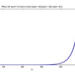
I am text block. Click edit button to change this text. Lorem ipsum dolor sit amet, consectetur adipiscing elit. Ut elit tellus, luctus nec ullamcorper mattis, pulvinar dapibus leo.
5.2. Second case: on the difference equation \(x_{n+1}= x_{n}+\dfrac{ x_{n} x_{n-4}}{ x_{n-3}-x_{n-4}}\)
In this subsection we study the following special case of Equation (1):Theorem 9. Let \(\{x_n\}_{n=-4}^\infty\) be a solution of Equation (7). Then for \(n=0,1,2,...\) \begin{equation*} \left\{ \begin{array}{llll} \displaystyle x_{8n-4}=\dfrac{r^{n}}{e^{n-1}}\dfrac{(rfgh)^{n}}{ (-f+e)^{n}(-g+f)^{n}(-h+g)^{n}(-r+h)^{n}}, & & & \\ \displaystyle x_{8n-3}=f\dfrac{r^{n}}{e^{n}}\dfrac{(rfgh)^{n}}{ (-f+e)^{n}(-g+f)^{n}(-h+g)^{n}(-r+h)^{n}}, & & & \\ \displaystyle x_{8n-2}=g\dfrac{r^{n}}{e^{n}}\dfrac{(rfgh)^{n}}{ (-f+e)^{n}(-g+f)^{n}(-h+g)^{n}(-r+h)^{n}}, & & & \\ \displaystyle x_{8n-1}=h\dfrac{r^{n}}{e^{n}}\dfrac{(rfgh)^{n}}{ (-f+e)^{n}(-g+f)^{n}(-h+g)^{n}(-r+h)^{n}}, & & & \\ \displaystyle x_{8n}=\dfrac{r^{n+1}}{e^n}\dfrac{(rfgh)^{n}}{ (-f+e)^{n}(-g+f)^{n}(-h+g)^{n}(-r+h)^{n}}, & & & \\ \displaystyle x_{8n+1}=-f\dfrac{r^{n+1}}{e^n}\dfrac{(rfgh)^{n}}{ (-f+e)^{n+1}(-g+f)^{n}(-h+g)^{n}(-r+h)^{n}}, & & & \\ \displaystyle x_{8n+2}=fg\dfrac{r^{n+1}}{e^n}\dfrac{(rfgh)^{n}}{ (-f+e)^{n+1}(-g+f)^{n+1}(-h+g)^{n}(-r+h)^{n}}, & & & \\ \displaystyle x_{8n+3}=-fgh\dfrac{r^{n+1}}{e^n}\dfrac{(rfgh)^{n}}{ (-f+e)^{n+1}(-g+f)^{n+1}(-h+g)^{n+1}(-r+h)^{n}}. & & & \end{array} \right. \end{equation*}
Proof. For \(n=0\), the result holds. Now suppose that our assumption holds for \(n-1\). That is \begin{equation*} \left\{ \begin{array}{llll} \displaystyle x_{8n-12}=\dfrac{r^{n-1}}{e^{n-2}}\dfrac{(rfgh)^{n-1}}{ (-f+e)^{n-1}(-g+f)^{n-1}(-h+g)^{n-1}(-r+h)^{n-1}}, & & & \\ \displaystyle x_{8n-11}=f\dfrac{r^{n-1}}{e^{n-1}}\dfrac{(rfgh)^{n-1}}{ (-f+e)^{n-1}(-g+f)^{n-1}(-h+g)^{n-1}(-r+h)^{n-1}}, & & & \\ \displaystyle x_{8n-10}=g\dfrac{r^{n-1}}{e^{n-1}}\dfrac{(rfgh)^{n-1}}{ (-f+e)^{n-1}(-g+f)^{n-1}(-h+g)^{n-1}(-r+h)^{n-1}}, & & & \\ \displaystyle x_{8n-9}=h\dfrac{r^{n-1}}{e^{n-1}}\dfrac{(rfgh)^{n-1}}{ (-f+e)^{n-1}(-g+f)^{n-1}(-h+g)^{n-1}(-r+h)^{n-1}}, & & & \\ \displaystyle x_{8n-8}=\dfrac{r^{n}}{e^{n-1}}\dfrac{(rfgh)^{n-1}}{ (-f+e)^{n-1}(-g+f)^{n-1}(-h+g)^{n-1}(-r+h)^{n-1}}, & & & \\ \displaystyle x_{8n-7}=-f\dfrac{r^{n}}{e^{n-1}}\dfrac{(rfgh)^{n-1}}{ (-f+e)^{n}(-g+f)^{n-1}(-h+g)^{n-1}(-r+h)^{n-1}}, & & & \\ \displaystyle x_{8n-6}=fg\dfrac{r^{n}}{e^{n-1}}\dfrac{(rfgh)^{n-1}}{ (-f+e)^{n}(-g+f)^{n}(-h+g)^{n-1}(-r+h)^{n-1}}, & & & \\ \displaystyle x_{8n-5}=-fgh\dfrac{r^{n}}{e^{n-1}}\dfrac{(rfgh)^{n-1}}{ (-f+e)^{n}(-g+f)^{n}(-h+g)^{n}(-r+h)^{n-1}}. & & & \end{array} \right. \end{equation*} Now it follows from Equation (7) that \begin{equation*} \begin{array}{llll} \displaystyle x_{8n}=\displaystyle x_{8n-1}+\dfrac{ x_{8n-1} x_{8n-5}}{ x_{8n-4}-x_{8n-5}}= h\dfrac{r^{n}}{e^{n}}\dfrac{(rfgh)^{n}}{ (-f+e)^{n}(-g+f)^{n}(-h+g)^{n}(-r+h)^{n}} & & & \\ \left(1+\dfrac{-fgh\dfrac{r^{n}}{e^{n-1}}\dfrac{(rfgh)^{n-1}}{ (-f+e)^{n}(-g+f)^{n}(-h+g)^{n}(-r+h)^{n-1}}}{\dfrac{r^{n}}{e^{n-1}}\dfrac{ (rfgh)^{n}}{(-f+e)^{n}(-g+f)^{n}(-h+g)^{n}(-r+h)^{n}}+fgh\dfrac{r^{n}}{ e^{n-1}}\dfrac{(rfgh)^{n-1}}{(-f+e)^{n}(-g+f)^{n}(-h+g)^{n}(-r+h)^{n-1}}} \right) & & & \\ =\displaystyle h\dfrac{r^{n}}{e^{n}}\dfrac{(rfgh)^{n}}{ (-f+e)^{n}(-g+f)^{n}(-h+g)^{n}(-r+h)^{n}} \left(1+\dfrac{-1}{\dfrac{r}{(-r+h) }+1}\right) \\ =\displaystyle h\dfrac{r^{n}}{e^{n}}\dfrac{(rfgh)^{n}}{ (-f+e)^{n}(-g+f)^{n}(-h+g)^{n}(-r+h)^{n}} \left(1+\dfrac{r-h}{h}\right) & & & \\ =\displaystyle h\dfrac{r^{n}}{e^{n}}\dfrac{(rfgh)^{n}}{ (-f+e)^{n}(-g+f)^{n}(-h+g)^{n}(-r+h)^{n}} \dfrac{r}{h}\\ =\displaystyle \dfrac{ r^{n+1}}{e^{n}}\dfrac{(rfgh)^{n}}{(-f+e)^{n}(-g+f)^{n}(-h+g)^{n}(-r+h)^{n}} & & & \end{array} \end{equation*} Similarly, \begin{equation*} \begin{array}{llll} \displaystyle x_{8n+1}=\displaystyle x_{8n}+\dfrac{ x_{8n} x_{8n-4}}{ x_{8n-3}-x_{8n-4}}\\ = \dfrac{r^{n+1}}{e^{n}}\dfrac{(rfgh)^{n}}{ (-f+e)^{n}(-g+f)^{n}(-h+g)^{n}(-r+h)^{n}} & & & \\ \left(1+\dfrac{\dfrac{r^{n}}{e^{n-1}}\dfrac{(rfgh)^{n}}{ (-f+e)^{n}(-g+f)^{n}(-h+g)^{n}(-r+h)^{n}}}{f\dfrac{r^{n}}{e^{n}}\dfrac{ (rfgh)^{n}}{(-f+e)^{n}(-g+f)^{n}(-h+g)^{n}(-r+h)^{n}}-\dfrac{r^{n}}{e^{n-1}} \dfrac{(rfgh)^{n}}{(-f+e)^{n}(-g+f)^{n}(-h+g)^{n}(-r+h)^{n}}}\right) & & & \\ =\displaystyle \dfrac{r^{n+1}}{e^{n}}\dfrac{(rfgh)^{n}}{ (-f+e)^{n}(-g+f)^{n}(-h+g)^{n}(-r+h)^{n}} \left(1+\dfrac{1}{\dfrac{f}{e}-1} \right)\\ =\displaystyle \dfrac{r^{n+1}}{e^{n}}\dfrac{(rfgh)^{n}}{ (-f+e)^{n}(-g+f)^{n}(-h+g)^{n}(-r+h)^{n}} \left(1+\dfrac{e}{f-e}\right) & & & \\ =\displaystyle \dfrac{r^{n+1}}{e^{n}}\dfrac{(rfgh)^{n}}{ (-f+e)^{n}(-g+f)^{n}(-h+g)^{n}(-r+h)^{n}} \dfrac{f}{f-e}\\ =\displaystyle -f \dfrac{r^{n+1}}{e^{n}}\dfrac{(rfgh)^{n}}{ (-f+e)^{n+1}(-g+f)^{n}(-h+g)^{n}(-r+h)^{n}} & & & \end{array} \end{equation*} Similarly, one can easily obtain the other relations. Thus, the proof is completed.
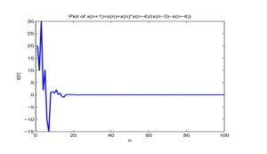
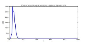
Consider numerical examples which represent different types of solutions to Equation (7).See Figure 3, since \(x_{-4}=20, x_{-3}=10, x_{-2}=30, x_{-1}=2, x_0=10\). The solution is bounded and converges to \(\bar x=0\).
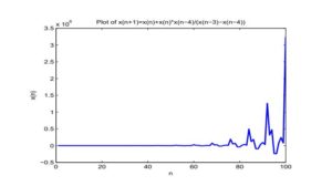
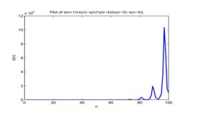
Now, if we take \(x_{-4}=1, x_{-3}=3, x_{-2}=1, x_{-1}=40, x_0=10\), the solution is unbounded (see Figure 4).
Figure 3. \(x_{-4}=20, x_{-3}=10, x_{-2}=30, x_{-1}=2, x_0=10\). The solution is bounded and converges to \(\bar x=0\).
Figure 4. \(x_{-4}=1, x_{-3}=3, x_{-2}=1, x_{-1}=40, x_0=10\), the solution is unbounded.
Theorem 10. Let \(\{x_n\}_{n=-4}^\infty\) be a solution of Equation (8). Then for \(n=0,1,2,...\) \begin{equation*} \left\{ \begin{array}{llll} \displaystyle x_{4n} & = & \dfrac{ r\;(rfgh)^n}{\displaystyle \prod_{i=1}^{n}(if+e)(ig+f)(ih+g)(ir+h)}, & \\ \displaystyle x_{4n+1} & = & \dfrac{ rf\;(rfgh)^n}{\displaystyle \prod_{i=1}^{n+1}(if+e)\prod_{i=1}^{n}(ig+f)(ih+g)(ir+h)}, & \\ \displaystyle x_{4n+2} & = & \dfrac{ rfg\;(rfgh)^n}{\displaystyle \prod_{i=1}^{n+1}(if+e)(ig+f)\prod_{i=1}^{n}(ih+g)(ir+h)}, & \\ \displaystyle x_{4n+3} & = & \dfrac{ (rfgh)^{n+1}}{\displaystyle \prod_{i=1}^{n+1}(if+e)(ig+f)(ih+g)\prod_{i=1}^{n}(ir+h)}. & \end{array} \right. \end{equation*}
Proof. For \(n=0\), the result holds. Now suppose that our assumption holds for \(n-1\) and for \(n-2\). That is \begin{equation*} \left\{ \begin{array}{llll} \displaystyle x_{4n-4} = \dfrac{ r\;(rfgh)^{n-1}}{\displaystyle \prod_{i=1}^{n-1}(if+e)(ig+f)(ih+g)(ir+h)}, & \\ \displaystyle x_{4n-3} = \dfrac{ rf\;(rfgh)^{n-1}}{\displaystyle \prod_{i=1}^{n}(if+e)\prod_{i=1}^{n-1}(ig+f)(ih+g)(ir+h)}, & \\ \displaystyle x_{4n-2} = \dfrac{ rfg\;(rfgh)^{n-1}}{\displaystyle \prod_{i=1}^{n}(if+e)(ig+f)\prod_{i=1}^{n-1}(ih+g)(ir+h)}, & \\ \displaystyle x_{4n-1} = \dfrac{ (rfgh)^{n}}{\displaystyle \prod_{i=1}^{n}(if+e)(ig+f)(ih+g)\prod_{i=1}^{n-1}(ir+h)}, & \end{array} \right. \left\{ \begin{array}{llll} \displaystyle x_{4n-8} = \dfrac{ r\;(rfgh)^{n-2}}{\displaystyle \prod_{i=1}^{n-2}(if+e)(ig+f)(ih+g)(ir+h)}, & \\ \displaystyle x_{4n-7} = \dfrac{ rf\;(rfgh)^{n-2}}{\displaystyle \prod_{i=1}^{n-1}(if+e)\prod_{i=1}^{n-2}(ig+f)(ih+g)(ir+h)}, & \\ \displaystyle x_{4n-6} = \dfrac{ rfg\;(rfgh)^{n-2}}{\displaystyle \prod_{i=1}^{n-1}(if+e)(ig+f)\prod_{i=1}^{n-2}(ih+g)(ir+h)}, & \\ \displaystyle x_{4n-5} = \dfrac{ (rfgh)^{n-1}}{\displaystyle \prod_{i=1}^{n-1}(if+e)(ig+f)(ih+g)\prod_{i=1}^{n-2}(ir+h)}. & \end{array} \right. \end{equation*} Now it follows from Equation (8) that \begin{equation*} \begin{array}{llll} \displaystyle x_{4n}=x_{4n-1}-\dfrac{ x_{4n-1} x_{4n-5}}{ x_{4n-4}+x_{4n-5}} = \dfrac{ (rfgh)^{n}}{\displaystyle \prod_{i=1}^{n}(if+e)(ig+f)(ih+g) \prod_{i=1}^{n-1}(ir+h)} & & & \\ \left(1-\dfrac{\dfrac{ (rfgh)^{n-1}}{\displaystyle \prod_{i=1}^{n-1}(if+e)(ig+f)(ih+g)\prod_{i=1}^{n-2}(ir+h)}}{\dfrac{ r\;(rfgh)^{n-1}}{\displaystyle \prod_{i=1}^{n-1}(if+e)(ig+f)(ih+g)(ir+h)} + \dfrac{ (rfgh)^{n-1}}{\displaystyle \prod_{i=1}^{n-1}(if+e)(ig+f)(ih+g) \prod_{i=1}^{n-2}(ir+h)}} \right) & & & \\ \end{array} \end{equation*} \begin{equation*} \begin{array}{llll}\displaystyle = \dfrac{ (rfgh)^{n}}{\displaystyle \prod_{i=1}^{n}(if+e)(ig+f)(ih+g)\prod_{i=1}^{n-1}(ir+h)} \left(1-\dfrac{1}{ \dfrac{ r}{(n-1)r+h} + 1} \right)\\ \displaystyle = \dfrac{ (rfgh)^{n}}{ \displaystyle \prod_{i=1}^{n}(if+e)(ig+f)(ih+g)\prod_{i=1}^{n-1}(ir+h)} \left(1-\dfrac{(n-1)r+h}{nr+h} \right) & & & \\ \displaystyle = \dfrac{ (rfgh)^{n}}{\displaystyle \prod_{i=1}^{n}(if+e)(ig+f)(ih+g)\prod_{i=1}^{n-1}(ir+h)} \left(\dfrac{r}{ nr+h} \right) \\ \displaystyle = \dfrac{ r(rfgh)^{n}}{\displaystyle \prod_{i=1}^{n}(if+e)(ig+f)(ih+g)(ir+h)} . & & & \\ \end{array} \end{equation*} Similarly, \begin{equation*} \begin{array}{llll} \displaystyle x_{4n+1}=x_{4n}-\dfrac{ x_{4n} x_{4n-4}}{ x_{4n-3}+x_{4n-4}}= \dfrac{ r(rfgh)^{n}}{\displaystyle \prod_{i=1}^{n}(if+e)(ig+f)(ih+g)(ir+h)} & & & \\ \left(1-\dfrac{\dfrac{ r(rfgh)^{n-1}}{\displaystyle \prod_{i=1}^{n-1}(if+e)(ig+f)(ih+g)(ir+h)}}{\dfrac{ rf\;(rfgh)^{n-1}}{ \displaystyle \prod_{i=1}^{n}(if+e)\prod_{i=1}^{n-1}(ig+f)(ih+g)(ir+h)} + \dfrac{ r(rfgh)^{n-1}}{\displaystyle \prod_{i=1}^{n-1}(if+e)(ig+f)(ih+g)(ir+h)}} \right) & & & \\ \end{array} \end{equation*} \begin{equation*} \begin{array}{llll} \displaystyle = \dfrac{r (rfgh)^{n}}{\displaystyle \prod_{i=1}^{n}(if+e)(ig+f)(ih+g)(ir+h)} \left(1-\dfrac{1}{\dfrac{ f}{nf+e} + 1} \right) \\ \displaystyle = \dfrac{ r(rfgh)^{n}}{\displaystyle \prod_{i=1}^{n}(if+e)(ig+f)(ih+g)(ir+h)} \left(1-\dfrac{nf+e}{(n+1)f+e} \right) & & & \\ \displaystyle = \dfrac{ r(rfgh)^{n}}{\displaystyle \prod_{i=1}^{n}(if+e)(ig+f)(ih+g)(ir+h)} \left(\dfrac{f}{(n+1)f+e} \right) \\ \displaystyle = \dfrac{ r(rfgh)^{n}}{\displaystyle \prod_{i=1}^{n+1}(if+e) \prod_{i=1}^{n}(ig+f)(ih+g)(ir+h)} . & & & \end{array} \end{equation*} Similarly, one can easily obtain the other relations. Thus, the proof is completed.
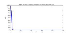
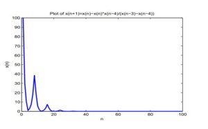
Consider numerical examples which represent different types of solutions to Equation (8).Assume that \(x_{-4}=100, x_{-3}=30, x_{-2}=80, x_{-1}=1, x_0=3\) (See Figure \ref{fig5}).
Now for \(x_{-4}=0.1, x_{-3}=0.5, x_{-2}=30, x_{-1}=50, x_0=300\) (See Figure \ref{fig6}).
Figure 6. \(x_{-4}=100, x_{-3}=30, x_{-2}=80, x_{-1}=1, x_0=3\).
Figure 6. \(x_{-4}=0.1, x_{-3}=0.5, x_{-2}=30, x_{-1}=50, x_0=300\).
5.3. Fourth case: on the difference equation \(x_{n+1}= x_{n}+\dfrac{ x_{n} x_{n-4}}{ -x_{n-3}+x_{n-4}}\)
In this subsection we study the following special case of Equation (1):Theorem 11. Let \(\{x_n\}_{n=-4}^\infty\) be a solution of Equation (9). Then for \(n=0,1,2,...\) \begin{equation*} \left\{ \begin{array}{llll} \displaystyle x_{8n-4}=\dfrac{r^{n}}{e^{n-1}}\dfrac{ (-f+2e)^{n}(-g+2f)^{n}(-h+2g)^{n}(-r+2h)^{n}}{ (-f+e)^{n}(-g+f)^{n}(-h+g)^{n}(-r+h)^{n}}, & & & \\ \displaystyle x_{8n-3}=f\dfrac{r^{n}}{e^{n}}\dfrac{ (-f+2e)^{n}(-g+2f)^{n}(-h+2g)^{n}(-r+2h)^{n}}{ (-f+e)^{n}(-g+f)^{n}(-h+g)^{n}(-r+h)^{n}}, & & & \\ \displaystyle x_{8n-2}=g\dfrac{r^{n}}{e^{n}}\dfrac{ (-f+2e)^{n}(-g+2f)^{n}(-h+2g)^{n}(-r+2h)^{n}}{ (-f+e)^{n}(-g+f)^{n}(-h+g)^{n}(-r+h)^{n}}, & & & \\ \displaystyle x_{8n-1}=h\dfrac{r^{n}}{e^{n}}\dfrac{ (-f+2e)^{n}(-g+2f)^{n}(-h+2g)^{n}(-r+2h)^{n}}{ (-f+e)^{n}(-g+f)^{n}(-h+g)^{n}(-r+h)^{n}}, & & & \\ \displaystyle x_{8n}=\dfrac{r^{n+1}}{e^n}\dfrac{ (-f+2e)^{n}(-g+2f)^{n}(-h+2g)^{n}(-r+2h)^{n}}{ (-f+e)^{n}(-g+f)^{n}(-h+g)^{n}(-r+h)^{n}} , & & & \\ \displaystyle x_{8n+1}=\dfrac{r^{n+1}}{e^n}\dfrac{ (-f+2e)^{n+1}(-g+2f)^{n}(-h+2g)^{n}(-r+2h)^{n}}{ (-f+e)^{n+1}(-g+f)^{n}(-h+g)^{n}(-r+h)^{n}}, & & & \\ \displaystyle x_{8n+2}=\dfrac{r^{n+1}}{e^n}\dfrac{ (-f+2e)^{n+1}(-g+2f)^{n+1}(-h+2g)^{n}(-r+2h)^{n}}{ (-f+e)^{n+1}(-g+f)^{n+1}(-h+g)^{n}(-r+h)^{n}}, & & & \\ \displaystyle x_{8n+3}=\dfrac{r^{n+1}}{e^n}\dfrac{ (-f+2e)^{n+1}(-g+2f)^{n+1}(-h+2g)^{n+1}(-r+2h)^{n}}{ (-f+e)^{n+1}(-g+f)^{n+1}(-h+g)^{n+1}(-r+h)^{n}}. & & & \end{array} \right. \end{equation*}
Proof. For \(n=0\), the result holds. Now suppose that our assumption holds for \(n-1\). That is \begin{equation*} \left\{ \begin{array}{llll} \displaystyle x_{8n-12}=\dfrac{r^{n-1}}{e^{n-2}}\dfrac{ (-f+2e)^{n-1}(-g+2f)^{n-1}(-h+2g)^{n-1}(-r+2h)^{n-1}}{ (-f+e)^{n-1}(-g+f)^{n-1}(-h+g)^{n-1}(-r+h)^{n-1}}, & & & \\ \displaystyle x_{8n-11}=f\dfrac{r^{n-1}}{e^{n-1}}\dfrac{ (-f+2e)^{n-1}(-g+2f)^{n-1}(-h+2g)^{n-1}(-r+2h)^{n-1}}{ (-f+e)^{n-1}(-g+f)^{n-1}(-h+g)^{n-1}(-r+h)^{n-1}}, & & & \\ \displaystyle x_{8n-10}=g\dfrac{r^{n-1}}{e^{n-1}}\dfrac{ (-f+2e)^{n-1}(-g+2f)^{n-1}(-h+2g)^{n-1}(-r+2h)^{n-1}}{ (-f+e)^{n-1}(-g+f)^{n-1}(-h+g)^{n-1}(-r+h)^{n-1}}, & & & \\ \displaystyle x_{8n-9}=h\dfrac{r^{n-1}}{e^{n-1}}\dfrac{ (-f+2e)^{n-1}(-g+2f)^{n-1}(-h+2g)^{n-1}(-r+2h)^{n-1}}{ (-f+e)^{n-1}(-g+f)^{n-1}(-h+g)^{n-1}(-r+h)^{n-1}}, & & & \\ \displaystyle x_{8n-8}=\dfrac{r^{n}}{e^{n-1}}\dfrac{ (-f+2e)^{n-1}(-g+2f)^{n-1}(-h+2g)^{n-1}(-r+2h)^{n-1}}{ (-f+e)^{n-1}(-g+f)^{n-1}(-h+g)^{n-1}(-r+h)^{n-1}} , & & & \\ \displaystyle x_{8n-7}=\dfrac{r^{n}}{e^{n-1}}\dfrac{ (-f+2e)^{n}(-g+2f)^{n-1}(-h+2g)^{n-1}(-r+2h)^{n-1}}{ (-f+e)^{n}(-g+f)^{n-1}(-h+g)^{n-1}(-r+h)^{n-1}}, & & & \\ \displaystyle x_{8n-6}=\dfrac{r^{n}}{e^{n-1}}\dfrac{ (-f+2e)^{n}(-g+2f)^{n}(-h+2g)^{n-1}(-r+2h)^{n-1}}{ (-f+e)^{n}(-g+f)^{n}(-h+g)^{n-1}(-r+h)^{n-1}}, & & & \\ \displaystyle x_{8n-5}=\dfrac{r^{n}}{e^{n-1}}\dfrac{ (-f+2e)^{n}(-g+2f)^{n}(-h+2g)^{n}(-r+2h)^{n-1}}{ (-f+e)^{n}(-g+f)^{n}(-h+g)^{n}(-r+h)^{n-1}}. & & & \end{array} \right. \end{equation*} Now it follows from Equation (9) that \begin{equation*} \begin{array}{llll} \displaystyle x_{8n}=x_{8n-1}+\dfrac{ x_{8n-1} x_{8n-5}}{-x_{8n-4}+x_{8n-5}} & & & \\ = h\dfrac{r^{n}}{e^{n}}\dfrac{(-f+2e)^{n}(-g+2f)^{n}(-h+2g)^{n}(-r+2h)^{n}}{ (-f+e)^{n}(-g+f)^{n}(-h+g)^{n}(-r+h)^{n}} & & & \\ \left(1+ \dfrac{\dfrac{r^{n}}{e^{n-1}}\dfrac{ (-f+2e)^{n}(-g+2f)^{n}(-h+2g)^{n}(-r+2h)^{n-1}}{ (-f+e)^{n}(-g+f)^{n}(-h+g)^{n}(-r+h)^{n-1}}}{-\dfrac{r^{n}}{e^{n-1}}\dfrac{ (-f+2e)^{n}(-g+2f)^{n}(-h+2g)^{n}(-r+2h)^{n}}{ (-f+e)^{n}(-g+f)^{n}(-h+g)^{n}(-r+h)^{n}}+\dfrac{r^{n}}{e^{n-1}}\dfrac{ (-f+2e)^{n}(-g+2f)^{n}(-h+2g)^{n}(-r+2h)^{n-1}}{ (-f+e)^{n}(-g+f)^{n}(-h+g)^{n}(-r+h)^{n-1}} }\right ) \\ \displaystyle = h \dfrac{r^{n}}{e^{n}}\dfrac{(-f+2e)^{n}(-g+2f)^{n}(-h+2g)^{n}(-r+2h)^{n}}{ (-f+e)^{n}(-g+f)^{n}(-h+g)^{n}(-r+h)^{n}} \left(1+ \dfrac{1}{-\dfrac{(-r+2h) }{(-r+h)}+1 }\right ) \\ \displaystyle = h\dfrac{r^{n}}{e^{n}}\dfrac{ (-f+2e)^{n}(-g+2f)^{n}(-h+2g)^{n}(-r+2h)^{n}}{ (-f+e)^{n}(-g+f)^{n}(-h+g)^{n}(-r+h)^{n}} \left(1+ \dfrac{(-r+h)}{-h}\right )\\ \displaystyle = h\dfrac{r^{n}}{e^{n}}\dfrac{ (-f+2e)^{n}(-g+2f)^{n}(-h+2g)^{n}(-r+2h)^{n}}{ (-f+e)^{n}(-g+f)^{n}(-h+g)^{n}(-r+h)^{n}} \left(\dfrac{r}{h}\right ) \\ \displaystyle = \dfrac{r^{n+1}}{e^{n}}\dfrac{ (-f+2e)^{n}(-g+2f)^{n}(-h+2g)^{n}(-r+2h)^{n}}{ (-f+e)^{n}(-g+f)^{n}(-h+g)^{n}(-r+h)^{n}}. \\ & & & \\ \displaystyle = h\dfrac{r^{n}}{e^{n}}\dfrac{ (-f+2e)^{n}(-g+2f)^{n}(-h+2g)^{n}(-r+2h)^{n}}{ (-f+e)^{n}(-g+f)^{n}(-h+g)^{n}(-r+h)^{n}} \left(1+ \dfrac{1}{-\dfrac{(-r+2h) }{(-r+h)}+1 }\right ) & & & \\ \displaystyle = h\dfrac{r^{n}}{e^{n}}\dfrac{ (-f+2e)^{n}(-g+2f)^{n}(-h+2g)^{n}(-r+2h)^{n}}{ (-f+e)^{n}(-g+f)^{n}(-h+g)^{n}(-r+h)^{n}} \left(1+ \dfrac{(-r+h)}{-h}\right )\\ \displaystyle = h\dfrac{r^{n}}{e^{n}}\dfrac{ (-f+2e)^{n}(-g+2f)^{n}(-h+2g)^{n}(-r+2h)^{n}}{ (-f+e)^{n}(-g+f)^{n}(-h+g)^{n}(-r+h)^{n}} \left(\dfrac{r}{h}\right ) & & & \\ \displaystyle = \dfrac{r^{n+1}}{e^{n}}\dfrac{ (-f+2e)^{n}(-g+2f)^{n}(-h+2g)^{n}(-r+2h)^{n}}{ (-f+e)^{n}(-g+f)^{n}(-h+g)^{n}(-r+h)^{n}}. & & & \end{array} \end{equation*} Similarly, \begin{equation*} \begin{array}{llll} \displaystyle x_{8n+1}=x_{8n}+\dfrac{ x_{8n} x_{8n-4}}{-x_{8n-3}+x_{8n-4}} = \dfrac{r^{n+1}}{e^{n}}\dfrac{(-f+2e)^{n}(-g+2f)^{n}(-h+2g)^{n}(-r+2h)^{n}}{ (-f+e)^{n}(-g+f)^{n}(-h+g)^{n}(-r+h)^{n}} & & & \\ \end{array} \end{equation*} \begin{equation*} \begin{array}{llll} \left(1+ \dfrac{\dfrac{r^{n}}{e^{n-1}}\dfrac{ (-f+2e)^{n}(-g+2f)^{n}(-h+2g)^{n}(-r+2h)^{n}}{ (-f+e)^{n}(-g+f)^{n}(-h+g)^{n}(-r+h)^{n}}}{-f\dfrac{r^{n}}{e^{n}}\dfrac{ (-f+2e)^{n}(-g+2f)^{n}(-h+2g)^{n}(-r+2h)^{n}}{ (-f+e)^{n}(-g+f)^{n}(-h+g)^{n}(-r+h)^{n}}+\dfrac{r^{n}}{e^{n-1}}\dfrac{ (-f+2e)^{n}(-g+2f)^{n}(-h+2g)^{n}(-r+2h)^{n}}{ (-f+e)^{n}(-g+f)^{n}(-h+g)^{n}(-r+h)^{n}} }\right ) \\ \displaystyle = \dfrac{ r^{n+1}}{e^{n}}\dfrac{(-f+2e)^{n}(-g+2f)^{n}(-h+2g)^{n}(-r+2h)^{n}}{ (-f+e)^{n}(-g+f)^{n}(-h+g)^{n}(-r+h)^{n}} \left(1+ \dfrac{1}{-\dfrac{f}{e}+1 }\right ) \\ \displaystyle = \dfrac{r^{n+1}}{e^{n}}\dfrac{ (-f+2e)^{n}(-g+2f)^{n}(-h+2g)^{n}(-r+2h)^{n}}{ (-f+e)^{n}(-g+f)^{n}(-h+g)^{n}(-r+h)^{n}} \left(1+ \dfrac{e}{-f+e}\right ) \\ \displaystyle = \dfrac{r^{n+1}}{e^{n}}\dfrac{ (-f+2e)^{n}(-g+2f)^{n}(-h+2g)^{n}(-r+2h)^{n}}{ (-f+e)^{n}(-g+f)^{n}(-h+g)^{n}(-r+h)^{n}} \left(\dfrac{-f+2e}{-f+e}\right ) \\ \displaystyle = \dfrac{r^{n+1}}{e^{n}}\dfrac{ (-f+2e)^{n+1}(-g+2f)^{n}(-h+2g)^{n}(-r+2h)^{n}}{ (-f+e)^{n+1}(-g+f)^{n}(-h+g)^{n}(-r+h)^{n}}\\ \displaystyle = \dfrac{r^{n+1}}{e^{n}}\dfrac{ (-f+2e)^{n}(-g+2f)^{n}(-h+2g)^{n}(-r+2h)^{n}}{ (-f+e)^{n}(-g+f)^{n}(-h+g)^{n}(-r+h)^{n}} \left(1+ \dfrac{1}{-\dfrac{f}{e}+1 }\right )\\ \displaystyle = \dfrac{r^{n+1}}{e^{n}}\dfrac{ (-f+2e)^{n}(-g+2f)^{n}(-h+2g)^{n}(-r+2h)^{n}}{ (-f+e)^{n}(-g+f)^{n}(-h+g)^{n}(-r+h)^{n}} \left(1+ \dfrac{e}{-f+e}\right ) & & & \\ \displaystyle = \dfrac{r^{n+1}}{e^{n}}\dfrac{ (-f+2e)^{n}(-g+2f)^{n}(-h+2g)^{n}(-r+2h)^{n}}{ (-f+e)^{n}(-g+f)^{n}(-h+g)^{n}(-r+h)^{n}} \left(\dfrac{-f+2e}{-f+e}\right ) \\ \displaystyle = \dfrac{r^{n+1}}{e^{n}}\dfrac{ (-f+2e)^{n+1}(-g+2f)^{n}(-h+2g)^{n}(-r+2h)^{n}}{ (-f+e)^{n+1}(-g+f)^{n}(-h+g)^{n}(-r+h)^{n}}. & & & \end{array} \end{equation*} Similarly, one can easily obtain the other relations. Thus, the proof is completed.
Consider numerical examples which represent different types of solutions to Equation (9).The solution is unbounded since we choose \(x_{-4}=20, x_{-3}=13, x_{-2}=3, x_{-1}=2, x_0=1\) (see Figure \ref{fig7}).
However the solution converges to \(\bar x=0\) by choosing \(x_{-4}=100, x_{-3}=30, x_{-2}=10, x_{-1}=1, x_0=3\) (see Figure \ref{fig8}).
Figure 7. The solution is unbounded since we choose \(x_{-4}=20, x_{-3}=13, x_{-2}=3,
x_{-1}=2, x_0=1\).
Figure 8. The solution converges to \(\bar x=0\) by choosing \(x_{-4}=100,
x_{-3}=30, x_{-2}=10, x_{-1}=1, x_0=3\)
6. Conclusion
This paper discussed global stability, boundedness, and the solutions of some special cases of Equation (1). In Section 2 we proved that if \( b(d+3c)< (1-a)(c+d)^{2}\) then the equilibrium point of Equation (1) is locally asymptotically stable. In Section 3 we showed that the unique equilibrium of Equation (1) is globally asymptotically stable if \(d(1-a)\not=b\). In Section 4 we proved that the solution of Equation (1) is bounded if \(a+\dfrac{b}{d}< 1\). In Section 5 we gave the form of the solution of four special cases of Equation (1) and gave numerical examples of each case.Author Contributions
All authors contributed equally to the writing of this paper. All authors read and approved the final manuscript.Conflicts of Interest:
The authors declare no conflict of interest.References
- El Hajji M. (2019). Analysis of a fractional-order "SVEIR" epidemic model with a general nonlinear saturated incidence rate in a continuous reactor. Asian Research Journal of Mathematics, 12(4), 1-17. [Google Scholor]
- El Hajji M. (2019). Global analysis of an epidemic mathematical model in a chemostat. Journal of Computer Science and Systems Biology, 4(1):103. [Google Scholor]
- El Hajji M. (2019). How the competitive exclusion principle can be validated using optical density measurements collected on artificially reconstituted soil ecosystems. Open Journal of Environmental Biology, 4(1), 001-006.[Google Scholor]
- El Hajji, M. (2019). Mathematical analysis of a fractional-order ``SIR" epidemic model with a general nonlinear saturated incidence rate in a chemostat. Asian Research Journal of Mathematics, 12(2), 1-12.[Google Scholor]
- El Hajji, M. (2019). Optimal control of an "SIR" epidemic model in a chemostat using some suitable protein doses. Journal of Advances in Mathematics and Computer Science, 30(6), 1-15.[Google Scholor]
- El Hajji, M. (2018). Boundedness and asymptotic stability of nonlinear Volterra integro-differential equations using Lyapunov functional. Journal of King Saud University - Science, https://doi.org/10.1016/j.jksus.2018.11.012.[Google Scholor]
- El Hajji M. (2018). How can inter-specific interferences explain coexistence or confirm the competitive exclusion principle in a chemostat. International Journal of Biomathematics, 11(8), 1850111.[Google Scholor]
- El Hajji, M., Chorfi N., & Jleli M. (2017). Mathematical modelling and analysis for a three-tiered microbial food web in a chemostat. Electronic Journal of Differential Equations, 255, 1-13.[Google Scholor]
- El Hajji, M., Chorfi N., & Jleli M. (2015). Mathematical model for a membrane bioreactor process. Electronic Journal of Differential Equations, 315, 1-7.[Google Scholor]
- El Hajji, M., Rapaport, A. (2010). Design of a cascade observer for a model of bacterial batch culture with nutrient recycling. IFAC Proceedings Volumes, 43(6), 203-208.[Google Scholor]
- El Hajji, M., Mazenc, F., & Harmand, J. (2010). A mathematical study of a syntrophic relationship of a model of anaerobic digestion process. Mathematical Biosciences & Engineering, 7(3), 641-656.[Google Scholor]
- El Hajji, M., & Rapaport A. (2009). Practical coexistence of two species in the chemostat - A slow-fast characterization. Mathematical Biosciences, 218(1), 33-39.[Google Scholor]
- El Hajji, M., Harmand, J., Chaker H., & Lobry, C. (2009). Association between competition and obligate mutualism in a chemostat. Journal of Biological Dynamics, 3(6), 635-647. [Google Scholor]
- Sari, T., El Hajji, M., & Harmand, J. (2012). The mathematical analysis of a syntrophic relationship between two microbial species in a chemostat. Mathematical Biosciences & Engineering, 9(1), 627-645.[Google Scholor]
- Sayari, S., & El Hajji M. (2019). fHow the fractional-order improve and extend the well-known competitive exclusion principle in the chemostat model with $n$ species competing for a single resource. Asian Research Journal of Mathematics, 12(3), 1-12.[Google Scholor]
- Abu Alhalawa, A., & Salah, M. (2017). Dynamics of higher order rational difference equation. International Journal of Nonlinear Analysis & Applications, 8(2), 363-379.[Google Scholor]
- Ahmed A.M., & Youssef, A.M. (2013). A solution form of a class of higher-order rational difference equations. Journal of the Egyptian Mathematical Society, 21, 248-253.[Google Scholor]
- Aloqeili, M. (2006). Dynamics of a rational difference equation. Applied Mathematics & Computation, 176(2), 768-774. [Google Scholor]
- Battaloglu, N., Cinar, C., & Yalc cinkaya, I. (2010). The Dynamics of the Difference Equation. Ars Combinatoria, 97, 281-288.[Google Scholor]
- Belhannache, F., Touafek, N., & Abo-Zeid, R. (2016). On a higher-order rational difference equation. Journal of Applied Mathematics & Informatics, 34(5-6), 369-382.[Google Scholor]
- Bozkurt, F., Ozturk I., & Ozen, S. (2009). )The global behavior of the difference equation. Studia Universitatis Babe¸s-Bolyai $/$ Mathematica, 54(2), 3-12.[Google Scholor]
- Cinar, C. (2004). On the positive solutions of the difference equation \(x_{n+1}=\dfrac{x_{n-1}}{1+ax_{n}x_{n-1}}\). Applied Mathematics & Computation, 158(3), 809-812.[Google Scholor]
- Cinar, C. (2004). On the solutions of the difference equation \(x_{n+1}=\dfrac{x_{n-1}}{-1+ax_{n}x_{n-1}}\). Applied Mathematics & Computation, 158(3), 793-797.[Google Scholor]
- Cinar, C. (2004). On the positive solutions of the difference equation \(x_{n+1}=\dfrac{ax_{n-1}}{1+bx_{n}x_{n-1}}\). Applied Mathematics & Computation, 156(2), 587-590.[Google Scholor]
- Elabbasy, E.M., & Elsayed, E.M. (2009). Dynamics of a rational difference equation. Chinese Annals of Mathematics, Series B, 30, 187-198.[Google Scholor]
- Elabbasy, E.M., El-Metwally, H., Elsayed, E.M. (2007). On the difference equations \(\displaystyle x_{n+1}=\dfrac{\alpha x_{n-k}}{\displaystyle \beta+\gamma\prod_{i=0}^k x_{n-i}}\). Journal of Computational & Applied Mathematics, 5(2), 101-113.[Google Scholor]
- \bibitem{12} Elabbasy, E.M., El-Metwally, H., & Elsayed, E.M. (2006). On the difference equation \(\displaystyle x_{n+1}=ax_n-\dfrac{bx_{n}}{cx_n-dx_{n-1}} \). Advances in Difference Equations, Article ID 82579, 1-10. [Google Scholor]
- El-Dessoky, M.M. (2017). On the difference equation \( x_{n+1}=ax_{n-1}+bx_{n-k}+\dfrac{cx_{n-s}}{dx_{n-s}-e}\). Mathematical Methods in the Applied Sciences, 40, 535-545.[Google Scholor]
- El-Metwally, H., & Elsayed, E.M. (2013). Form of solutions and periodicity for systems of difference equations. Journal of Computational Analysis \& Applications, 15(5), 852-857. [Google Scholor]
- Elsayed, E.M. (2013). Behavior and Expression of the Solutions of Some Rational Difference Equations. Journal of Computational Analysis & Applications, 15(1), 73-81.[Google Scholor]
- Elsayed, E.M. (2010). Qualitative properties for a fourth order rational difference equation. Acta Applicandae Mathematicae, 110(2), 589-604.[Google Scholor]
- Elsayed, E.M. (2010). On the Global attractivity and the solution of recursive sequence. Studia Scientiarum Mathematicarum Hungarica, 47(3), 401-418.[Google Scholor]
- Elsayed, E.M. (2009). Qualitative behavior of difference equation of order three. Acta Scientiarum Mathematicarum (Szeged), 75(1-2), 113-129. [Google Scholor]
- Elsayed, E.M. (2009). Dynamics of a rational recursive sequence. International Journal of Differential Equations, 4(2), 185-200.[Google Scholor]
- Elsayed, E.M. (2008). Qualitative behavior of s rational recursive sequence. Indagationes Mathematicae, New Series, 19(2), 189-201.[Google Scholor]
- Elsayed, E.M., Alzahrani, F., & Alayachi, H.S. (2018). Formulas and properties of some class of nonlinear difference equations. Journal of Computational Analysis & Applications, 24(8), 1517-1531.[Google Scholor]
- Elsayed, E.M., & Khaliq, A. (2016). The Dynamics and Global attractivity of a Rational Difference Equation. Advanced Studies in Contemporary Mathematics, 26(1), 183-202. [Google Scholor]
- Kocic V.L., & Ladas, G. (1993). Global Behavior of Nonlinear Difference Equations of Higher Order with Applications. Kluwer Academic Publishers, Dordrecht.[Google Scholor]
- Kulenovic M.R.S., & Ladas, G. (2001). Dynamics of Second Order Rational Difference Equations with Open Problems and Conjectures. Chapman & Hall / CRC Press.[Google Scholor]
- Liu, K., Li, P., Han F., & Zhong, W. (2018). Global Dynamics of Nonlinear Difference Equation \(x_{n+1} = \dfrac{x_n}{x_{n-1} x_{n-2}} \). Journal of Computational Analysis & Applications, 24(6), 1125-1132.[Google Scholor]
- Ocalan, O., Ogunmez, H., & Gumus, M. (2014). Global behavior test for a non-linear difference equation with a period-two coefficient. Dynamics of Continuous, Discrete & Impulsive Systems Series A: Mathematical Analysis, 21, 307-316. [Google Scholor]
- Saleh, M., & Abu-Baha, S. (2006). Dynamics of a higher order rational difference equation. Applied Mathematics & Computation, 181(1), 84-102.[Google Scholor]
- Simsek, D., Cinar, C., & Yalcinkaya, I. (2006). On the recursive sequence \(x_{n+1}=\dfrac{x_{n-3}}{1+x_{n-1}}\). International Journal of Contemporary Mathematical Sciences, 1(10), 475-480.[Google Scholor]
- Sun, T., Zhou, Y., Su, G., & Bin Qin, (2018). Eventual periodicity of a max-type difference equation system. Journal of Computational Analysis & Applications, 24(5), 976-983.[Google Scholor]
- Wang, C.Y., Fang X.J., & Li, R. (2016). On the solution for a system of two rational difference equations. Journal of Computational Analysis & Applications, 20(1), 175-186. [Google Scholor]
- Wang, C.Y., Fang, X.J., & Li, R. (2017). On the dynamics of a certain four-order fractional difference equations. Journal of Computational Analysis & Applications, 22(5), 968-976.[Google Scholor]
- Wang, C., Zhou, Y., Pan S., & Li, R. (2018). On a system of three max-type nonlinear difference equations. Journal of Computational Analysis & Applications, 25(8), 1463-1479.[Google Scholor]
- Ibrahim, T.F. (2017). Closed Form Expressions of some systems of Nonlinear Partial Difference Equations. Journal of Computational Analysis & Applications, 23(3), 433-445.[Google Scholor]

