Complex dynamics of a fractional-order predator-prey interaction with harvesting

1. Introduction

Fractional differential equations are more suitable for modeling many real-life phenomena than ordinary differential equations. Fractional calculus has seen significant development over the past few decades. Chaos is a very interesting nonlinear phenomenon which has been intensively studied due to its useful applications in science and technology [1,2,3]. Studying chaos in fractional-order dynamical systems is an interesting topic as well. The discrete fractional equations recently attracted researchers in the modeling of the biological populations and interaction of the species [4,5,6,7]. Harvesting has a strong impact on the dynamic evolution of a population subjected to it. The effects of predator harvesting were reported in [8,9], harvesting among two fish species and its effects were studied in [10].

In this paper, the predator-prey model is considered with harvesting effort affecting both species directly. We studied the following fractional-order predator-prey model.

By using discretization of fractional order using piecewise constant arguments methods [11,12] to (1) fractional model we have the following discrete model where \(0< \alpha \leq 1\) is the fractional-order and \(k\) is the step size of discretization, \(x(t)\) is the population of prey at time \(t\), \(y(t)\) is the population of predator at time \(t\), \(a\) is the rate of growth of prey, \(b\) is the interaction rate, \(c\) is the constant harvesting effort of prey, \(d\) is the mortality rate of predator, \(e\) is the conversion rate of prey, \(f\) is the constant harvesting effort of predator. All parameters are assumed to be positive.

The paper is organized as follows. In Section 2, we investigate the topological classification of the unique positive equilibrium point of the system (2). In Section 3, we discuss period-doubling bifurcation and in Section 4, we discuss Neimark-Sacker bifurcation at positive steady-state. In Section 5, some numerical examples are presented to verify our theoretical results. In Section 6, some concluding remarks are presented.

2. Local stability of positive equilibrium point

The system (2) has three equilibrium points. \[ E_0\left(0,0\right), E_1\left(\frac{a-c}{a},0\right), E_2\left(\frac{d+f}{e},\frac{ae-ad-af-ce}{be}\right). \] Note that if \(ae-ad-af-ce>0\), then \(E_2\) is the unique positive equilibrium point of (2). \(E_0\) is the mutual extinction, \(E_1\) is the predator extinction and \(E_3\) is coexistence equilibrium point of system (2). For bilogically meaningful we concentrated on coexistence equilibrium point \(E_2\). The jacobian matrix of (2) evaluated at \(E_2\) is given by \[ J(E_2)= \begin{bmatrix} 1-\frac{aM(d+f)}{e} & \frac{-bM(d+f)}{e} \\ -\frac{(ce+a(d-e+f))M}{b} & 1 \end{bmatrix}, \] where \(M=\frac{k^{\alpha}}{\Gamma({\alpha+1})}\). The corresponding characteristic polynomial is By simple computations we have \begin{eqnarray*} F(0)&=&1+M^2(d+f)(a-c)-\frac{aM(d+f)(1+M(d+f))}{e}, \\ F(1)&=&\frac{M^2(d+f)(ae-ad-af-ce)}{e}, \\ F(-1)&=&4+M^2(d+f)(a-c)-\frac{aM(d+f)(2+M(d+f))}{e}. \end{eqnarray*} Since \(ae-ad-af-ce>0\), therefore \(F(1)>0\). For stability analysis we use the following result.

Lemma 1. [13]: Let \(F(\lambda)=\lambda^2-A \lambda+B\), where \(A, B\) are constants. Suppose \(F(1)>0\) and \(\lambda_1, \lambda_2\) are roots of \(F(\lambda)=0\), then

• (i) \(|\lambda_1|< 1\) and \(|\lambda_2|< 1\) iff \(F(-1)>0\) and \(F(0)< 1\).
• (ii) \(|\lambda_1|< 1\) and \(|\lambda_2|>1\) iff \(F(-1)< 0\).
• (iii) \(|\lambda_1|>1\) and \(|\lambda_2|>1\) iff \(F(-1)>0\) and \(F(0)>1\).
• (iv) \(\lambda_1=-1\) and \(|\lambda_2|\neq 1\) iff \(F(-1)=0\) and \(F(0)\neq \pm 1\).
• (v) \(\lambda_1\) and \(\lambda_2\) are complex and \(|\lambda_1|=|\lambda_2|=1\) iff \(A^2-4B< 0\) and \(F(0)=1\).

Theorem 1. If \((a,b,c,d,e,f,M)\in \mathbb{R}_+^7, \ ae-ad-af-ce>0\) and \(\lambda_1, \lambda_2\) are the roots of \(F(\lambda)=0\) given by (3), then

• (i) \(|\lambda_1|< 1\) and \(|\lambda_2|< 1\) iff \[ a-\frac{a(1+dM+fM)}{eM}< c< a+\frac{4}{(d+f)M^2}-\frac{a(2+dM+fM)}{eM}, \]
• (ii) \(|\lambda_1|< 1\) and \(|\lambda_2|>1\) iff \[ c>a+\frac{4}{(d+f)M^2}-\frac{a(2+dM+fM)}{eM}, \]
• (iii) \(|\lambda_1|>1\) and \(|\lambda_2|>1\) iff \[ c< min \lbrace a-\frac{a(1+dM+fM)}{eM}, a+\frac{4}{(d+f)M^2}-\frac{a(2+dM+fM)}{eM} \rbrace, \]
• (iv) \(\lambda_1=-1\) and \(|\lambda_2|\neq 1\) iff \[ c=a+\frac{4}{(d+f)M^2}-\frac{a(2+dM+fM)}{eM}, \ c \neq a-\frac{a(1+dM+fM)}{eM}, \ c \neq a+\frac{2}{(d+f)M^2}-\frac{a(1+dM+fM)}{eM}, \]
• (v) \(\lambda_1\) and \(\lambda_2\) are complex and \(|\lambda_1|=|\lambda_2|=1\) iff \[ c=a-\frac{a(1+dM+fM)}{eM}, \ \frac{a(d+f)M}{e}< 4. \]
The following corollary is an immediate consequence of Theorem 1.

Corollary 1. If \((a,b,c,d,e,f,M)\in \mathbb{R}_+^7, \ ae-ad-af-ce>0\), then the unique positive equilibrium point \(E_2\) of (2) is:

• (i) a sink and therefore locally asymptotically stable if \[ a-\frac{a(1+dM+fM)}{eM}< c< a+\frac{4}{(d+f)M^2}-\frac{a(2+dM+fM)}{eM}, \]
• (ii) saddle point and therefore unstable if \[ c>a+\frac{4}{(d+f)M^2}-\frac{a(2+dM+fM)}{eM}, \]
• (iii) source or repeller and therefore unstable if \[ c< min \left\lbrace a-\frac{a(1+dM+fM)}{eM}, a+\frac{4}{(d+f)M^2}-\frac{a(2+dM+fM)}{eM} \right\rbrace, \] and
• (iv) non-hyperbolic if \[ c=a+\frac{4}{(d+f)M^2}-\frac{a(2+dM+fM)}{eM}, \ c \neq a-\frac{a(1+dM+fM)}{eM}, \ c \neq a+\frac{2}{(d+f)M^2}-\frac{a(1+dM+fM)}{eM}, \] or \[ c=a-\frac{a(1+dM+fM)}{eM}, \ \frac{a(d+f)M}{e}< 4. \]

3. Period doubling bifurcation

In this section, we investigate that system (2) undergoes period doubling bifurcation [14,15] at the positive equilibrium point \(E_2\). Consider \begin{eqnarray*} \Lambda&=&\left\lbrace (a,b,c,d,e,f,M) \in \mathbb{R}^7_+\right. \Big| ae-ad-af-ce>0,\;\; c=a+\frac{4}{(d+f)M^2}-\frac{a(2+dM+fM)}{eM}, \\&& c \neq a-\frac{a(1+dM+fM)}{eM},\;\; c \neq a+\frac{2}{(d+f)M^2}\left.-\frac{a(1+dM+fM)}{eM} \right\rbrace. \end{eqnarray*} We discuss the period doubling bifurcation of the system (2) at \(E_2\) when parameters vary in a small neighborhood of \(\Lambda\). Taking \(c\) as bifurcation parameter, we consider a perturbation of the system (2) as follows:
\begin{equation} \label{PD} \begin{cases} x(t+1)=x(t)+M\left[ax(t)(1-x(t))-bx(t)y(t)-(c+\delta)x(t)\right], \\ y(t+1)=y(t)+M\left[-dy(t)+ex(t)y(t)-fy(t)\right], \end{cases} \end{equation}
(4)
where \(M=\frac{k^{\alpha}}{\Gamma({\alpha+1})}\) and \(|\delta| \ll 1\) is small perturbation parameter.

We define a transformation by \(\xi(t)=x(t)-\frac{d+f}{e}\) and \(\eta(t)=y(t)-\frac{a(e-d-f)-(c+\delta)e}{be}\) to transfer the equilibrium point \(E_2\) to \((0,0)\). Under this transformation system (4) will become

\begin{equation} \label{PD1} \begin{bmatrix} \xi(t+1) \\ \eta(t+1) \end{bmatrix}= \begin{bmatrix} a_{11} & a_{12} \\ a_{21} &1 \end{bmatrix} \begin{bmatrix} \xi(t) \\ \eta(t) \end{bmatrix}+ \begin{bmatrix} a_1 \xi^2(t)+a_2 \xi(t) \eta(t) \\ b_1 \xi(t) \delta+b_2 \xi(t) \eta(t) \end{bmatrix}, \end{equation}
(5)
where \( a_{11}=1-\frac{a(d+f)M}{e} , \ a_{12}=-\frac{bM(d+f)}{e}, \ a_{21}=\frac{2(aM(d+f)-2e)}{bM(d+f)}, a_1=-a M, \ a_2= -bM, \ b_1=-\frac{eM}{b}, \ b_2=eM. \) Eigenvalues of linearized part of (5) are \(-1\) and \(\lambda=3-\frac{aM(d+f)}{e}\). We construct an invertible matrix \(T\) as \( T=\begin{bmatrix} \frac{bM(d+f)}{2e-aM(d+f)} & -\frac{bM(d+f)}{2e} \\ 1 & 1 \end{bmatrix}. \) Now we apply the transformation \( \begin{bmatrix} \xi(t) \\ \eta(t) \end{bmatrix}= T \begin{bmatrix} u(t) \\ v(t) \end{bmatrix}, \) to the system (5) and we get
\begin{equation} \label{PD2} \begin{bmatrix} u(t+1) \\ v(t+1) \end{bmatrix}= \begin{bmatrix} -1 & 0 \\ 0 & \lambda \end{bmatrix} \begin{bmatrix} u(t) \\ v(t) \end{bmatrix}+ \begin{bmatrix} F(u(t),v(t),\delta) \\ G(u(t),v(t),\delta) \end{bmatrix}, \end{equation}
(6)
where \begin{eqnarray*} F(u(t),v(t),\delta)=a_1 u^2(t)+a_2 v^2(t)+a_3 u(t)v(t)+a_4 u(t) \delta+a_5 v(t) \delta, \\ G(u(t),v(t),\delta)=b_1 u^2(t)+b_2 v^2(t)+b_3 u(t) v(t)+b_4 u(t) \delta+b_5 v(t) \delta, \end{eqnarray*} with \begin{align*} a_1&=\frac{beM(-aM^2(d+f)^2+2e(-2+dM+fM))}{(2e-a(d+f)M)(4e-a(d+f)M)}, \\ a_2&=\frac{bM(-2e+a(d+f)M)(a(d+f)M+e(-2+dM+fM))}{2e(4e-a(d+f)M)}, \\ a_3&=\frac{ab(d+f)M^2(2+dM+fM)}{8e-2a(d+f)M} ,\\ a_4&=\frac{e(d+f)M^2}{aM(d+f)-4e}, \\ a_5&=-\frac{(d+f)M^2(-2e+a(d+f)M)}{8e-2a(d+f)M},\\ b_1&=\frac{2be^2M(2+dM+fM)}{(2e-a(d+f)M)(4e-a(d+f)M)}, \\ b_2&=-\frac{bM(-4ae(d+f)M+a^2(d+f)^2M^2+2e^2(2+dM+fM))}{2e(4e-a(d+f)M)}, \\ b_3&=\frac{ab(d+f)M^2(a(d+f)M+e(-2+dM+fM))}{(2e-a(d+f)M)(4e-a(d+f)M)},\\ b_4&=-\frac{2e^2M^2(d+f)}{(2e-a(d+f)M)(4e-a(d+f)M)}, \\ b_5&=\frac{e(d+f)M^2}{4e-a(d+f)M}. \end{align*} Next we determine the center manifold \(W^c(0,0)\) of the system (6) at the equilibrium point \((0,0)\) in a small neighbourhood of \(\delta=0\). By using center manifold theory [16,17,18], we know that there exist a center manifold \(W^c(0,0)\), which can be approximately represented as follows: \[ W^c(0,0)=\left\lbrace (u(t),v(t)) \in \mathbb{R}^2 \vert v(t)=W(u(t),\delta)=m_1 u^2(t)+m_2 \delta u(t) +m_3 \delta^2+ O ((|u(t)|+|\delta|)^3) \right\rbrace. \] By using first equation of system (6), we have
\begin{align} v(t+1)=W(u(t+1),\delta)=-m_2 \delta u(t)+m_1 u^2(t)+m_3 \delta^2+O((|u(t)|+|\delta|)^3). \label{PD3} \end{align}
(7)
By using second equation of system (6), we have
\begin{align} v(t+1)=\lambda v(t)+G(u(t),v(t),\delta)=(b_4+\lambda m_2) \delta u(t)+(b_1+\lambda m_1)u^2(t)+\lambda m_3 \delta^2+O((|u(t)|+|\delta|)^3). \label{PD4} \end{align}
(8)
Comparing the coefficients for (7) and (8), we have \[ m_1=\frac{b_1}{1-\lambda}, \ m_2=-\frac{b_4}{1+\lambda}, \ m_3=0.\] Then the center manifold can be approximated as follows
\begin{equation} \label{PD5} v(t)=\frac{b_1}{1-\lambda}u^2(t)-\frac{b_4}{1+\lambda}\delta u(t)+O((|u(t)|+|\delta|)^3). \end{equation}
(9)
Substituting (9) in the first equation of the system (6), we have \begin{align} u(t+1)&=-u(t)+a_1 u^2(t)+a_4 u(t) \delta+\frac{a_3 b_1}{1-\lambda} u^3(t)+ (\frac{a_5 b_1}{1-\lambda}-\frac{a_3 b_4}{1+\lambda}) u^2(t) \delta \nonumber \\ & \;\;\;-\frac{a_5 b_4}{1+\lambda} u(t) \delta^2+O((|u(t)|+|\delta|)^3)=\tilde{F}(u(t),\delta). \nonumber \end{align} For period doubling bifurcation we need the following two quantities \[ L=\left( \frac{\partial^2 \tilde{F}}{\partial u(t) \partial \delta} +\frac{1}{2}\frac{\partial \tilde{F}}{\partial \delta} \frac{\partial^2 \tilde{F}}{\partial u^2(t)}\right)_{u(t)=0,\delta=0}, \] and \[ M=\left(\frac{1}{6}\frac{\partial^3 \tilde{F}}{\partial u^3(t)}+\left(\frac{1}{2}\frac{\partial^2 \tilde{F}}{\partial u^2(t)}\right)^2 \right)_{u(t)=0,\delta=0}. \] By simple computations, we have \[ L=a_4 , \ M=a_1^2+\frac{a_3b_1}{1-\lambda}. \] By using above calculations we have the following result for period doubling bifurcation of the system (2).

Theorem 2. If \((a,b,c,d,e,f,M)\in \Lambda\) and \(L \neq 0, M \neq 0\) then the system (2) goes under period doubling bifurcation at the equilibrium point \(E_2\). Moreover, if \(M>0\) (or \(M< 0\)) then period-2 orbits that bifurcate from the equilibrium point \(E_2\) are stable (or unstable).

4. Neimark-Sacker bifurcation

In this section, we investigate that system (2) undergoes Neimark-Sacker bifurcation [19,20] at the positive equilibrium point \(E_2\). Consider \[ \Omega=\left\lbrace (a,b,c,d,e,f,M) \in \mathbb{R}^7_+ \mid ae-ad-af-ce>0, \ c=a-\frac{a(1+dM+fM)}{eM}, \ \frac{a(d+f)M}{e}< 4 \right\rbrace, \] where \(M=\frac{k^{\alpha}}{\Gamma(\alpha+1)}\).

We discuss the Neimark-Sacker bifurcation of the system (2) at \(E_2\) when parameters vary in a small neighbourhood of \(\Omega\). Taking \(c\) as bifurcation parameter, we consider a perturbation of the system (2) as follows:

\begin{equation} \label{NS1} \begin{cases} x(t+1)=x(t)+M\left[ax(t)(1-x(t))-bx(t)y(t)-(c+\delta)x(t)\right], \\ y(t+1)=y(t)+M\left[-dy(t)+ex(t)y(t)-fy(t)\right], \end{cases} \end{equation}
(10)
where \(M=\frac{k^{\alpha}}{\Gamma({\alpha+1})}\) and \(|\delta| \ll 1\) is small perturbation parameter.

We define a transformation by \(\xi(t)=x(t)-\frac{d+f}{e}\) and \(\eta(t)=y(t)-\frac{a(e-d-f)-(c+\delta)e}{be}\) to transfer the equilibrium point \(E_2\) to \((0,0)\). Under this transformation system (10) will become

\begin{equation} \label{NS2} \begin{bmatrix} \xi(t+1) \\ \eta(t+1) \end{bmatrix}= \begin{bmatrix} a_{11} & a_{12} \\ a_{21} & 1 \end{bmatrix} \begin{bmatrix} \xi(t) \\ \eta(t) \end{bmatrix}+ \begin{bmatrix} -bM \xi(t) \eta(t)-aM \xi^2(t) \\ eM \xi(t) \eta(t) \end{bmatrix}, \end{equation}
(11)
where \( a_{11}=1-\frac{aM(d+f)}{e}, \ a_{12}=-\frac{bM(d+f)}{e}, \ a_{21}=\frac{a-eM \delta}{b}. \)

The characteristic equation of the linearized part of the system (11) at equilibrium point \((0,0)\) is

\begin{equation} \label{NS3} \lambda^2-p(\delta) \lambda+q(\delta)=0, \end{equation}
(12)
where \(p(\delta)=2-\frac{aM(d+f)}{e}, \) and \( q(\delta)=1-dM^2 \delta-fM^2 \delta. \)

The roots of (12) are complex with \(|\lambda_{1,2}|=1\) which are given by \( \lambda_{1,2}=\frac{p(\delta)\pm i \sqrt{4q(\delta)-p^2(\delta)}}{2}. \) By computations, we obtain \( |\lambda_1|=|\lambda_2|=\sqrt{q(\delta)}, \) and \( \left(\frac{d|\lambda_1|}{d \delta}\right)_{\delta=0}=\left(\frac{d|\lambda_2|}{d \delta}\right)_{\delta=0}=-\frac{(d+f)M^2}{2}< 0. \)

By simple computations, we can check that \(p(0)=2-\frac{a(d+f)M}{e}\). Since \(\frac{a(d+f)M}{e}< 4\), therefore we have \(-2< p(0)< 2\). If we set \(p(0)=0\), then we obtain \(\frac{a(d+f)M}{e}=2\) and if we set \(p(0)=1\), then we obtain \(\frac{a(d+f)M}{e}=1\). Since \(\lambda_1^m,\lambda_2^m \neq1\) for \(m=1,2,3,4\) at \(\delta=0\) is equivalent to \(p(0) \neq \pm 2, 0,1\), therefore \(\lambda_1^m,\lambda_2^m \neq1\) for \(m=1,2,3,4\) at \(\delta=0\) if \((a,b,c,d,e,f,M)\in \Omega\) and following conditions are satisfied:

\begin{equation} \label{NS3A} \frac{a(d+f)M}{e} \neq 1, 2. \end{equation}
(13)
Now we use the following transformation to convert the linear part of (11) into its canonical form at \(\delta=0\).
\begin{equation} \label{NS4} \begin{bmatrix} \xi(t) \\ \eta(t) \end{bmatrix}= \begin{bmatrix} -\frac{b(d+f)M}{e} & 0 \\ \frac{aM(d+f)}{2e} & -\frac{1}{2} \sqrt{4-(-2+\frac{aM(d+f)}{e})^2} \end{bmatrix} \begin{bmatrix} u(t) \\ v(t) \end{bmatrix}. \end{equation}
(14)
Under the transformation (14), the system (11) will become
\begin{equation} \label{NS5} \begin{bmatrix} u(t+1) \\ v(t+1) \end{bmatrix}= \begin{bmatrix} \alpha & -\beta \\ \beta & \alpha \end{bmatrix} \begin{bmatrix} u(t) \\ v(t) \end{bmatrix}+ \begin{bmatrix} f(u(t),v(t)) \\ g(u(t),v(t)) \end{bmatrix}, \end{equation}
(15)
where \begin{align*} \alpha&=1-\frac{aM(d+f)}{2e}, \\ \beta&=\frac{1}{2}\sqrt{4-(-2+\frac{aM(d+f)}{e})^2}, \\ f(u,v)&=\frac{abM^2(d+f)}{2e} u^2+\frac{bM}{2}\sqrt{4-(-2+\frac{aM(d+f)}{e})^2} u v, \\ g(u,v)&=\frac{abM^3(a+2e)(d+f)^2}{2e\sqrt{aM(d+f)(4e-aM(d+f))}} u^2+\frac{b(a-2e)(d+f)M^2}{2e} u v. \end{align*} We define the following real number \(L\), which analyses the direction in which the closed invariant curve occurs in a system undergoing Neimark-Sacker bifurcation method: \[L=\left( \left[-Re \left( \frac{(1-2 \lambda_1)\lambda_2^2}{1-\lambda_1}\eta_{20}\eta_{11} \right) - \frac{1}{2} \vert \eta_{11} \vert^2 - \vert \eta_{02} \vert^2 + Re(\lambda_2 \eta_{21}) \right] \right)_{\delta=0},\] where \begin{align*} \eta_{20}&=\frac{1}{8}\left[ f_{uu} - f_{vv} + 2g_{uv} + i (g_{uu} - g_{vv} -2f_{uv})\right], \\ \eta_{11}&=\frac{1}{4}\left[ f_{uu} + f_{vv} + i (g_{uu} + g_{vv})\right], \\ \eta_{02}&=\frac{1}{8}\left[ f_{uu} - f_{vv} - 2g_{uv} + i (g_{uu} - g_{vv} + 2f_{uv})\right], \\ \eta_{21}&=\frac{1}{16}\left[ f_{uuu} + f_{uvv} + f_{uuv} + g_{vvv} + i (g_{uuu} + g_{uvv} - f_{uuv} - f_{vvv})\right]. \end{align*} From calculations the computed partial derivatives are \begin{align*} f_{uu}&=\frac{abM^2(d+f)}{e}, \\ f_{uv}&=\frac{bM}{2}\sqrt{4-(-2+\frac{aM(d+f)}{e})^2}, \\ f_{vv}&=f_{uuu}=f_{vvv}=f_{uvv}=f_{uuv}=0, \\ g_{vv}&=g_{uuu}=g_{vvv}=g_{uvv}=g_{uuv}=0, \\ g_{uu}&=\frac{abM^3(a+2e)(d+f)^2}{e\sqrt{aM(d+f)(4e-aM(d+f))}}, \\ g_{uv}&=\frac{bM^2(d+f)(a-2e)}{2e}. \end{align*} Due to above calculations, we have the following result for existence and direction of Neimark-Sacker bifurcation.

Theorem 3. Assume that \((a,b,c,d,e,f,M)\in \Omega\) and conditions (13) are satisfied. If \(L \neq 0\), then the system (2) goes under Neimark-Sacker bifurcation at the unique positive equilibrium point \(E_2\) when the parameter \(c\) varies in a small neighbourhood of \(c=a-\frac{a(1+dM+fM)}{eM}\). Furthermore, if \(L< 0\), then an attracting invariant closed curve bifurcates from the equilibrium point for \(c>a-\frac{a(1+dM+fM)}{eM}\), and if \(L>0\), then a repelling invariant closed curve bifurcates from the equilibrium point for \(c< a-\frac{a(1+dM+fM)}{eM}\).

5. Numerical examples

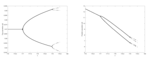
In this section some interesting numerical examples are provided to validate our theoretical discussions on various qualitative aspects of the model.

Example 1. We select the parameters values as \(a=200, b=0.8, d=2.3, e=40,f=0.5, k=0.15,\alpha=0.95\) and initial conditions \(x(0)=0.1, y(0)=8\). For these values the unique positive equilibrium point of (2) is \((0.07,11.2316)\). The eigenvalues of \(J(E_2)\) for these values are \(\lambda_1=-1, \lambda_2=0.643641\), which confirms that the system (2) undergoes period doubling bifurcation at \((0.07,11.2316)\) as bifurcation parameter passes through \(c=177.015\). We plot bifurcation diagrams for both prey and predator populations for \(c \in [176,180]\). (see Figure 1)

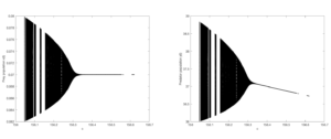
Example 2. We select the parameters values as \(a=200, b=0.8, d=2.3, e=40,f=0.5, k=0.15,\alpha=0.95\) and initial conditions \(x(0)=0.1, y(0)=35\). For these values the unique positive equilibrium point of (2) is \((0.07,37.1336)\). The eigenvalues of \(J(E_2)\) for these values are \(\lambda_1=-0.17818+0.983998i, \lambda_2=-0.17818-0.983998i\) with \(|\lambda_{1,2}|=1\), which confirms that the system (2) undergoes Neimark-Sacker bifurcation at \((0.07,37.1336)\) as bifurcation parameter passes through \(c=156.293\). We plot bifurcation diagrams for both prey and predator populations for \(c \in [156,156.7]\). (see Figure 2 )

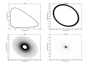
Example 3. We select the parameters values as \(a=20, b=10, d=2, e=40, f=1, k=0.11, \alpha=0.9\) and the initial conditions \(x(0)=0.073, y(0)=0.35\). The positive equilibrium point for these values is \((0.075,0.35058)\). For these values the equilibrium point is locally asymptotically stable iff \(14.9942< c< 77.0381\). We plot phase portraits for \(c=14, 14.9942, 15, 15.2 \). Clearly one can see that for \(c=14\), the equilibrium point \((0.35058,0.142621)\) is unstable, whereas for \(c=15\) and \(c=15.2\) it is stable. For \(c=14.9942\), the system undergoes bifurcation. (See figure 3 )

6. Conclusion

We studied a fractional-order predator-prey model with harvesting in both species. We study the existence and local stability of coexistence equilibrium point \(E_2\) of system (2) and their dependence in the form of constant harvesting effort of prey. Moreover, the system (2) goes under period-doubling bifurcation and Neimark-Sacker bifurcation under certain conditions on constant harvesting effort of prey. Numerical examples are presented to support our theoretical results.

conflictofinterests

The author declares no conflict of interest.