Engineering and Applied Science Letter
ISSN: 2617-9709 (Online) 2617-9695 (Print)
DOI: 10.30538/psrp-easl2019.0027
Analytical solution of isotropic rectangular plates resting on Winkler and Pasternak foundations using Laplace transform and variation of iteration method
M. G. Sobamowo, O. M. Sadiq, S. A. Salawu\(^1\)
Department of Mechanical Engineering, University of Lagos, Akoka, Lagos, Nigeria.; (M.G.S)
Department of Civil and Environmental Engineering, University of Lagos, Akoka, Nigeria.; ( O.S & S.S)
Abstract
Keywords:
1. Introduction
Research into vibration analysis of thin isotropic rectangular plate resting on elastic nonlinear foundation is vast gaining significant awareness among researchers due to its wide applications and important in the field of engineering. Geotechnics engineers need to understand the behaviour of plates when embedded in soil for their design, structural engineers requires same information for the design of the structural foundations likewise highway engineers rely on the information for the highway pavement design. In the design of elastic soil foundation, the adoption of two- parameter foundations gives better results than the use of Winkler foundation alone, which is associated with limitation of shear interaction among the spring elements. In the study of dynamic behavior of plates, Jain et al. [1] worked on free vibration of rectangular plate. In another work, natural frequency of rectangular plate was determined by Bhat [2] using Rayleight method. Few years later, Balkaya [3] investigated the dynamic response of rectangular plate using differential transform method (DTM). Thereafter, Gupta et al. [4] analyzed forced vibration of rectangular plate with varying thickness. In a further study, some other researchers [5, 6, 7, 8, 9, 10] studied buckling and vibration of plates and beams.
Several authors already applied different method of solutions for analysis of thin rectangular plate. However, in numerical analysis [9, 10, 11, 12, 13, 14, 15, 16, 17, 18, 19, 20, 21, 22, 23], it is very important to carry out convergence and stability study which increases the computational time and cost otherwise the solution will diverge. Furthermore, exact method [24, 25, 26] are having the limitation of handling nonlinear problem due to the complex mathematics involved. These limitations had led to the introduction of semi-analytical methods. Ozturk and Coskun [27] used Homotopy perturbation method (HPM) in the study of plate dynamic behaviour. However, despite the effectiveness, there is setback of finding embedded parameters. In another study, Galerkin method of solution was adopted by Njoku [28] for vibration analysis of thin isotropic rectangular plate. The method suffers the limitation of extension of the series solution to provide precise result. In a later work, Pirbodaghi et al.[29] utilized Homotopy analysis method (HAM) for investigation of vibration analysis of beam. HAM suffers from limitation of assumption of solution for the expression. Variation of iteration method (VIM), was first proposed by He [30,31, 32, 33, 34, 35, 36], has been applied to investigate many nonlinear partial differential equation. The approach uses Lagrange multiplier to find the analytical solution with very fast convergence. This present study adopts the use of exact method to handle the linear part of the system governing equation and solving the rest of equation with very effective method of VIM. The advantage of this method over other hybrid method calls for its application in this research.
Despite the effectiveness of the method and high prediction of results, the author realized that, with several researches on dynamic analysis of plate, Laplace transform and VIM has not been used to determine analytical solution of thin rectangular isotropic plate resting on two-parameter foundations. Therefore, the present study is on determination of analytical solution of free vibration of thin isotropic rectangular plate resting on nonlinear foundation. The analytical solution obtained is used for investigation of the controlling parameters.
2. Problem formulation and mathematical analysis
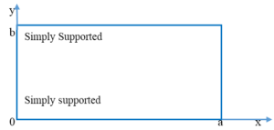
Considering homogenous rectangular plate of uniform thickness resting on Winkler and Pasternak foundations as shown in Figure 2. The two opposite edge \(y=0\) and \(y=b\) are regarded as simply supported.Figure 1. Rectangular plate resting on two-parameter foundations
Figure 2. Geometry of plate with boundary conditions
- Normal stresses in the direction transverse to the plate are considered small.
- Thickness of plate is smaller compared to the other dimensions.
- Plate is of constant thickness.
- Normal to the undeformed middle surface remains straight and unstretched in length and still normal to the deformed middle surface.
The governing equation for thin isotropic rectangular plate as reported by Leissa [38] is;
2.1. Boundary conditions
Three boundary conditions are considered at \(X = 0\) and \(X = l\) namely, Simply supported and clamped edge (SC), Simply supported and simply supported edge (SS) and Simply supported and free edge conditions (SF).3. Method of Solution: Laplace transform and variation iteration method
3.1. Basic ideal of Laplace transform
If \(f(t)\) is a function of a variable \(t\). \(\mathscr{L}{F(t)}\) and is defined by the integral:
\begin{equation}
\mathscr{L}\{F(t)\} = f(s) = \int_{0}^{\infty}e^{-st}F(t)dt.
\label{equ11}
\end{equation}
(11)
Some of the properties used in this study include:
\begin{equation}
\mathscr{L}\{1\} = \frac{1}{s} (s \ge 0),
\label{equ12}
\end{equation}
(12)
\begin{equation}
\mathscr{L}\{t^{n}\} = \frac{n!}{s^{n+1}}(s \ge 0),
\label{equ13}
\end{equation}
(13)
\begin{equation}
\mathscr{L}\{F^{n}(t)\} = n^{n}f(s) - s^{n-1}F(0) - s^{n-2}F'(0) \dots F^{n-1}(0),
\label{equ14}
\end{equation}
(14)
where \(F^{n}(t)\) represents the \(n-th\) derivative of \(F(t)\) and \(\mathscr{L}\{F(t)\} = f(s)\). If Laplace transform of \(F(t)\) is \(f(s)\), then the inverse Laplace transform of \(f(s)\) is expressed as \(F(t) = \mathscr{L^{-1}}\{f(s)\}\), where \(\mathscr{L^{-1}}\) is called inverse Laplace operator. The inverse Laplace of Equations (12) and (13) are:
\begin{equation}
1 = \mathscr{L^{-1}} \frac{1}{s},
\label{equ15}
\end{equation}
(15)
\begin{equation}
t^{n} = \mathscr{L^{-1}} \bigg(\frac{n!}{s^{n+1}}\bigg),
\label{equ16}
\end{equation}
(16)
3.2. Laplace and variation iteration method
Assuming the following nonlinear differential equation:
\begin{equation}
Lw(x) + Nw(x) = f,
\label{equ17}
\end{equation}
(17)
\(L\) represents the linear operator, \(N\) is nonlinear operator, \(f\) is the source or analytical function. VariatiFon iteration method use the correction function for Equation (17) as:
\begin{equation}
w_{n+1}(x) = w_{n}(x) + \int_{0}^{x} \lambda(\zeta) \big[Lw_{n}(\zeta)+ N \tilde{w_{n}}(\zeta) - f(\zeta) \big] d \zeta, \ \ n =0, 1, 2, \dots,
\label{equ18}
\end{equation}
(18)
where \(\lambda\) is general Lagrange multiplier identified through variational theory. The subscript \(n\) represents the \(nth\) term and \(\tilde{w_{n}}\) is a constrained variation \((\delta \tilde{w_{n}} = 0) \).
Laplace transform of both sides of Equation (12) gives:
\begin{equation}
\mathscr{L}\big[w_{n+1}(x)\big] = \mathscr{L}\big[w_{n}(x)\big] + \mathscr{L}\bigg[\int_{0}^{x} \bar{\lambda}(x - \zeta) \big[Lw_{n}(\zeta)+ N \tilde{w_{n}}(\zeta) - f(\zeta) \big] d \zeta] \bigg], \ \ \ n = 0, 1, 2, \dots
\label{equ19}
\end{equation}
(19)
Apply convolution to Equation (19), we get
\begin{eqnarray}
\mathscr{L}\big[w_{n+1}(x)\big] &=& \mathscr{L}\big[w_{n}(x)\big] + \mathscr{L} \bigg[\bar{\lambda}(x) \times \big[Lw_{n}(x)+ N \tilde{w_{n}}(x) - f(x)\big]\bigg] \nonumber \\
&=& \mathscr{L}\big[w_{n}(x)\big] + \mathscr{L} \bigg[\bar{\lambda}(x) \mathscr{L} \big[Lw_{n}(x)+ N \tilde{w_{n}}(x) - f(x)\big]\bigg]. \label{equ20}
\end{eqnarray}
(20)
Optimal value of \(\bar{\lambda}(x - \zeta)\) is obtained taking variation with respect to \(w_{n}(x)\) given as;
\begin{equation}
\frac{\delta}{\delta w_{n}}\mathscr{L} \big[w_{n+1}(x)\big] = \frac{\delta}{\delta w_{n}}\mathscr{L} \big[w_{n}(x)\big] + \frac{\delta}{\delta w_{n}}\mathscr{L} \big[\bar{\lambda}(x)\big] \mathscr{L} \big[Lw_{n}(x)+ N \tilde{w_{n}}(x) - f(x)\big].
\label{equ21}
\end{equation}
(21)
Applying variation with respect to \(w_{n}(x)\) gives:
\begin{equation}
\mathscr{L}\big[\delta w_{n+1}\big] = \mathscr{L} \big[\delta w_{n}\big] + \delta \mathscr{L} \big[\bar{\lambda}\big] \mathscr{L}\big[w_{n}\big].
\label{equ22}
\end{equation}
(22)
Assume \(L\) is linear differential operator with constant coefficients as;
\begin{equation}
L(w) = a_{0}w + a_{1}w' + a_{2}w''+ \dots + a_{n-2}w^{n-2} + a_{n-1}w^{n-1} + a_{n}w^{n}
\label{equ23}
\end{equation}
(23)
where \(a_{i}'s\) are constants. The coefficient contains non-constant terms of the form \(x^{k}\). The Laplace transform of initial operator term is given as:
\begin{equation}
\mathscr{L}\big[a_{n}w^{n} \big] = a_{n}s^{n}\mathscr{L}\big[w \big] - a_{n} \sum_{k=1}^{n}s^{k-1}w^{n-k}(0).
\label{equ24}
\end{equation}
(24)
The variation with respect to \(w\) is given as:
\begin{equation}
\mathscr{L} \big[\delta w_{n+1}\big] = \mathscr{L} \big[\delta w_{n}\big] + \mathscr{L}\big[\bar{\lambda}\big]\bigg[\sum_{k=0}^{n}a_{k}s^{k} \bigg] \mathscr{L} \big[\delta w_{n}\big] = \bigg[ 1+ \mathscr{L}\big[\bar{\lambda}\big] \bigg[\sum_{k=0}^{n}a_{k}s^{k} \bigg] \bigg] \mathscr{L}\big[\delta w_{n}\big].
\label{equ25}
\end{equation}
(25)
Extremum condition \(w_{n+1}\) needs that \(\delta w_{n+1}\). Meaning the right hand side of Equation (25) should be set to zero. Hence stationary condition is;
\begin{equation}
\mathscr{L}\big[\bar{\lambda}\big] = -\frac{1}{\sum\limits_{k=0}^{n}a_{k}s^{k}}.
\label{equ26}
\end{equation}
(26)
3.3. Application of LVIM to the governing equation
Following the basic principle of LVIM , the governing equation is now analyzed as:
\begin{eqnarray}
\mathscr{L}\big[w_{n+1}(x)\big]&=& \mathscr{L}\big[w_{n}(x)\big] + \mathscr{L}\big[\bar{\lambda}\big] \mathscr{L} \bigg[\frac{d^{4}W_{n}(X)}{dX^{4}} - 2 \lambda^{2} m^{2} \pi^{2} \frac{d^{2}W_{n}(x)}{dX^{2}}\nonumber \\
&&- (\Omega^{2}- k_{w} - \lambda^{4} m^{4} \pi^{4})W_{n}(x) - k_{p}W^{3}_{n}(x) \bigg] \nonumber \\
&=& \mathscr{L}\big[w_{n}(x)\big] + \mathscr{L}\big[\bar{\lambda}\big] \bigg[(\lambda^{4} m^{4} \pi^{4} - 2 \pi^{2} s^{2} \lambda^{2} m^{2} + s^{2} - \Omega^{2} + k_{w})\mathscr{L}\big[w_{n}(x)\big]\nonumber\\
&&-w_{n}''(0) - sw_{n}''(0) - s^{2}w_{n}'(0) - s^{3}w_{n}(0) + 2 m^{2} \lambda^{2}\pi^{2}w_{n}(0) + sw_{n}(0) -k_{p} \mathscr{L} \big[ W^{3}(x)\big] \bigg].
\label{equ27}
\end{eqnarray}
(27)
Taking variation with respect to \(w_{n}(x)\) on both sides of Equation (27), we get
\begin{eqnarray}
\frac{\delta}{\delta w_{n}}\mathscr{L} \big[w_{n+1}(x)\big] &=& \frac{\delta}{\delta w_{n}}\mathscr{L} \big[w_{n}(x)\big] + \frac{\delta}{\delta w_{n}}\mathscr{L} \big[\bar{\lambda(x)}\big] \bigg[(\lambda^{4} m^{4} \pi^{4} - 2 \pi^{2} s^{2} \lambda^{2} m^{2} + s^{2} - \Omega^{2} + k_{w})\mathscr{L}\big[w_{n}(x)\big] \nonumber \\
&&-w_{n}''(0)- sw_{n}''(0) - s^{2}w_{n}'(0) - s^{3}w_{n}(0) + 2 m^{2} \lambda^{2}\pi^{2}w_{n}(0) + sw_{n}(0) -k_{p} \mathscr{L}\big[W^{3}(x)\big] \bigg]\nonumber\\
&&
\label{equ28}
\end{eqnarray}
(28)
Simplifying Equation (28) gives,
\begin{eqnarray}
\mathscr{L}\big[\delta w_{n+1} \big] &=& \mathscr{L}\big[\delta w_{n} \big] + \mathscr{L}\big[\bar{\lambda}\big]\big((\lambda^{4} m^{4} \pi^{4} - 2 \pi^{2} s^{2} \lambda^{2} m^{2} + s^{2} - \Omega^{2} + k_{w})\mathscr{L}\big[\delta w_{n}\big]) \big) \nonumber \\
&=& \mathscr{L}\big[\delta w_{n} \big] \big(1 + \mathscr{L}\big[\bar{\lambda}\big](\lambda^{4} m^{4} \pi^{4} - 2 \pi^{2} s^{2} \lambda^{2} m^{2} + s^{2} - \Omega^{2} + k_{w}) \big)
\label{equ29}
\end{eqnarray}
(29)
Extremum condition \(w_{n+1}\) needs that \(\delta w_{n+1} = 0\) . Meaning the right hand side of Equation (29) should be set to zero.
\begin{equation}
1 + \mathscr{L}\big[\bar{\lambda}\big](\pi^{4} - 2 \pi^{2} s^{2} + s^{4}) = 0, \ \ \mathscr{L}\big[\bar{\lambda}\big] = -\frac{1}{\big( \pi^{4} - 2 \pi^{2} s^{2} + s^{4} \big)}.
\label{equ30}
\end{equation}
(30)
For simplicity we adopt,
\begin{equation}
\mathscr{L}\big[\bar{\lambda}\big] = -\frac{1}{s^{4}}.
\label{equ31}
\end{equation}
(31)
Substituting Equation (31) into Equation (27) results;
\begin{eqnarray}
\mathscr{L}\big[ w_{n+1}(x) \big] &=& \mathscr{L}\big[ w_{n}(x) \big] - \mathscr{L} \bigg[\int_{0}^{x} \bar{\lambda} (x- \zeta) \bigg[ \frac{d^{4}W_{n}(\zeta)}{d\zeta^{4}} - 2m^{2} \pi^{2} \lambda^{2} \frac{d^{2}W_{n}(\zeta)}{d\zeta^{2}} \nonumber \\
&&- \big( \Omega^{2} -m^{4} \pi^{4} \lambda^{4} -k_{w} \big)W_{n}(\zeta) - k_{p}W^{3}_{n}(\zeta) \bigg] d \zeta \bigg] \nonumber \\
&=& \mathscr{L}\big[ w_{n}(x) \big] - \mathscr{L} \bigg[\frac{x^{3}}{6}\bigg] \mathscr{L}\bigg[ \frac{d^{4}W_{n}(\zeta)}{d\zeta^{4}} - 2m^{2} \pi^{2} \lambda^{2} \frac{d^{2}W_{n}(\zeta)}{d\zeta^{2}} \nonumber \\
&&- \big( \Omega^{2} -m^{4} \pi^{4} \lambda^{4} - k_{w}\big)W_{n}(x) - k_{p}W^{3}_{n}(x) \bigg].
\label{equ32}
\end{eqnarray}
(32)
Assuming
\begin{eqnarray}
\Phi_{0} =
\begin{cases}
w(0), & \text{if}\; L = \frac{d}{dx} \\
w(0) + xw'(0), & \text{if}\; L = \frac{d^{2}}{dx^{2}} \\
w(0) + xw'(0) + \frac{x^{2}}{2!}w''(0), & \text{if} \; L = \frac{d^{3}}{dx^{3}} \\
w(0) + xw'(0) + \frac{x^{2}}{2!}w''(0) + \frac{x^{3}}{3!}w'''(0), & \text{if} \; L = \frac{d^{4}}{dx^{4}} ,\\
\end{cases}
\label{equ33}
\end{eqnarray}
(33)
\begin{equation}
w_{0} = w(0) + w'(0)x + \frac{1}{2!}w''(0)x^2 + \frac{1}{3!}w'''(0)x^{3}.
\label{equ34}
\end{equation}
(34)
Applying condition (9) at \(x = 0\) on Equation (34) gives
\begin{equation}
w_{0} = w'(0)x + \frac{1}{3!}w'''(0)x^{3} = ax + \frac{\beta}{3!}x^{3!}.
\label{equ35}
\end{equation}
(35)
Then
\begin{equation}
\mathscr{L}\big[ w_{1} \big] = \mathscr{L}\big[ w_{0} \big] - \mathscr{L} \bigg[\frac{x^{3}}{6}\bigg] \mathscr{L}\bigg[ \frac{d^{4}W_{0}(x)}{dX^{4}} - 2m^{2} \pi^{2} \lambda^{2} \frac{d^{2}W_{0}(x)}{dX^{2}} - \big( \Omega^{2} -m^{4} \pi^{4} \lambda^{4} - k_{w} \big)W_{0}(x) - k_{p}W^{3}_{0}(x) \bigg].
\label{equ36}
\end{equation}
(36)
\begin{equation}
\mathscr{L}\big[ w_{1} \big] = \frac{\alpha s^{2} + \beta}{s^{4}} - \frac{1}{s^{4}} \bigg[\frac{(-m^{4} \pi^{4} \lambda^{4}+ \Omega^{2}- k_{w})(\alpha s^{2} + \beta)}{s^{4}} + \frac{k_{p}(\alpha s^{2} + \beta)^{3}}{s^{12}} \bigg].
\label{equ37}
\end{equation}
(37)
Inverse Laplace gives the first iteration:
\begin{eqnarray}
w_{1} &=& \bigg[-259459200\pi^{4}\beta\lambda^{4}m^{4}x^{2} + \beta^{3}k_{p}x^{10} - 10897286400 \pi^{4}\alpha \lambda^{4}m^{4} + 630 \alpha \beta^{2}k_{p}x^{8} \nonumber \\
&&+ 98280 \alpha^{2} \beta k_{p}x^{6} + 3603600 \alpha^{3} k_{p}x^{4} + 259459200 \Omega^{2}\beta x^{2} \nonumber \\
&&- 259459200 \beta k_{w}x^{2} + 10897286400 \Omega^{2} \alpha - 10897286400 \alpha k_{w}\bigg]\frac{x^{5}}{1307674368000} + \frac{1}{6}x(\beta x^{2}+ 6 \alpha),
\label{equ38}
\end{eqnarray}
(38)
\begin{equation}
\mathscr{L}\big[w_{2}\big] = \mathscr{L}\big[w_{1}\big] - \mathscr{L} \bigg[\frac{x^{3}}{6}\bigg] \mathscr{L}\bigg[ \frac{d^{4}W_{1}(x)}{dX^{4}} - 2m^{2} \pi^{2} \lambda^{2} \frac{d^{2}W_{1}(x)}{dX^{2}} - \big( \Omega^{2} -m^{4} \pi^{4} \lambda^{4} - k_{w} \big)W_{x} - k_{p}W^{3}_{1}(x) \bigg],
\label{equ39}
\end{equation}
(39)
\begin{eqnarray}
&&\mathscr{L}\big[w_{2}\big] = \mathscr{L}\big[w_{1}\big] - \frac{1}{s^{4}} \bigg[ \big( \Omega^{2} -m^{4} \pi^{4} \lambda^{4} - k_{w} \big) \bigg( -\frac{\pi^{4} \beta \lambda^{4} m^{4}}{s^{8}} + \frac{\Omega^{2}\beta}{s^{8}} - \frac{\beta k_{w}}{s^{8}} - \frac{\pi^{4} \alpha \lambda^{4}m^{4}}{s^{6}} + \frac{\Omega^{2}\alpha}{s^{6}} -\frac{\alpha k_{w}}{s^{6}} \nonumber \\
&&+\frac{3 \alpha^{2} \beta k_{p}}{s^{12}}+\frac{\alpha^{3} k_{p}}{s^{10}} + \frac{3 \alpha \beta^{2} k_{p}}{s^{14}} +\frac{\beta^{3} k_{p}}{s^{16}} + \frac{\beta}{s^{4}} + \frac{\alpha}{s^{2}} \bigg) + k_{p}\bigg( -\frac{\pi^{4} \beta \lambda^{4} m^{4}}{s^{8}} + \frac{\Omega^{2}\beta}{s^{8}} - \frac{\beta k_{w}}{s^{8}} - \frac{\pi^{4} \alpha \lambda^{4}m^{4}}{s^{6}} + \frac{\Omega^{2}\alpha}{s^{6}} \nonumber \\
&&-\frac{\alpha k_{w}}{s^{6}} +\frac{3 \alpha^{2} \beta k_{p}}{s^{12}} +\frac{\alpha^{3} k_{p}}{s^{10}} + \frac{3 \alpha \beta^{2} k_{p}}{s^{14}} +\frac{\beta^{3} k_{p}}{s^{16}} + \frac{\beta}{s^{4}} + \frac{\alpha}{s^{2}} \bigg) \bigg].
\label{equ40}
\end{eqnarray}
(40)
Inverse Laplace gives the second iteration:
\begin{eqnarray}
w_{2} &=& \bigg[-1424499357221085171226298826358784000000 \pi^{12} \beta^{3}k_{p} \lambda^{12} m^{12} x^{22} \nonumber \\
&&+ 4503328777444754421964800000 \pi^{8} \beta^{5} k^{2}_{p} \lambda^{8} m^{8} x^{30} \nonumber \\
&&-299999564628605370602585328311599104000000 \pi^{12} \alpha \beta^{2} k_{p}\lambda^{12}m^{12}x^{20} \nonumber \\
&&- 77022858528000 \pi^{4} \beta^{7}k_{p}\lambda^{4}m^{4}x^{38}+ \dots \bigg] x^{5} + \frac{1}{3}x\big(\beta x^{2} + 6 \alpha \big) \nonumber \\
&&+ \bigg[-259459200 \pi^{4}\beta \lambda^{4}m^{4}x^{2} + \beta^{3}k_{p}x^{10} - 10897286400 \pi^{4}\alpha \lambda^{4} m^{4} \nonumber \\
&&+ 630 \alpha \beta^{2} k_{p} x^{8} 98280 \alpha^{2} \beta k_{p} x^{6} -3603600 \alpha^{3}k_{p} x^{4} + 259459200 \Omega^{2}\beta x^{2} -259459200 \beta k_{w} x^{2} \nonumber \\
&& + 10897286400 \Omega^{2} \alpha - 10897286400 \alpha_{w} \bigg] \frac{x^{5}}{1307674368000},
\label{equ41}
\end{eqnarray}
(41)
The same approach is continued till frequency parameter \(\Omega\) obtained converges. Substituting boundary condition at \(x = 1\) to find the unknowns introduced results into simultaneous equation.
Table 1. Parameters for validation of the model.
Edge
Condition/Dimensionless
Simply-supported
(SS)
Simply supported
-Clamped (SC)
Simply-supported
-Free (SF)
Natural frequency
Bhat et al.;[2]
Present
Leissa [38]
Present
Leissa [38]
Present
\(\Omega 1\)
19.7392
19.7434
23.6463
23.6486
11.7195
11.7606
Table 1 contains parameters for validation of the approach to ascertain the correctness of the results.
\begin{align}
\psi^{n}_{11}(\Omega)w_{0} + \psi^{n}_{12}(\Omega)w_{2} \nonumber \\
\psi^{n}_{21}(\Omega)w_{0} + \psi^{n}_{22}(\Omega)w_{2}.
\label{equ42}
\end{align}
(42)
The polynomials are represented as \(\psi_{11}, \psi_{12}, \psi_{21}\) and \(\psi_{22}\). Equation (42) can be written in matrix form as:
\begin{eqnarray}
\begin{bmatrix}
\psi^{n}_{11}(\Omega) & \psi^{n}_{12}(\Omega) \\
\psi^{n}_{21}(\Omega) & \psi^{n}_{22}(\Omega)
\end{bmatrix}
\begin{bmatrix}
w_{0} \\
w_{2}
\end{bmatrix}
=
\begin{bmatrix}
0 \\
0
\end{bmatrix}
\label{equ43}
\end{eqnarray}
(43)
The following Characteristic determinant is obtained applying the non-trivial condition
\begin{eqnarray}
\begin{bmatrix}
\psi^{n}_{11}(\Omega) & \psi^{n}_{12}(\Omega) \\
\psi^{n}_{21}(\Omega) & \psi^{n}_{22}(\Omega)
\end{bmatrix}
=
\begin{bmatrix}
0 \\
0
\end{bmatrix}
\label{equ44}
\end{eqnarray}
(44)
Solving Equation (44) gives the natural frequencies. Substitute the result obtained into Equation (43), we get
\begin{eqnarray}
\begin{bmatrix}
\frac{245431}{40824} & \frac{32120}{19453} \\
\frac{-181919}{3773} & \frac{-125273}{9460}
\end{bmatrix}
\begin{bmatrix}
\alpha \\
\beta
\end{bmatrix}_{1}
=
\begin{bmatrix}
0 \\
0
\end{bmatrix}
\label{equ45}
\end{eqnarray}
(45)
Setting \(\alpha = 1\) and find \(\beta\)
\begin{eqnarray}
\begin{bmatrix}
\alpha \\
\beta
\end{bmatrix}_{1}
=
\begin{bmatrix}
1 \\
-3.641035489
\end{bmatrix}
\label{equ46}
\end{eqnarray}
(46)
Same procedure is repeated for other modes.
\begin{eqnarray}
w(x) &=& \bigg[\frac{4.27 \times 10^{58} \pi^{8} x^{4} - 2.36 \times 10^{60} x^{6} -3.34 \times 10^{62} x^4 - 4.58 \times 10^{62}x^{2} + 5.28 \times 10^{63} } {1.55 \times 10^{64}}\bigg] x^{5} \nonumber \\
&& - \frac{1}{3}\bigg[-\frac{47399}{13018}x^{2}- 6 \bigg]x - \bigg[\frac{3.86 \times 10^{8} x^{2} -4.45 \times 10^{9}}{1.30 \times 10^{10}}\bigg]x^{5}
\label{equ47}
\end{eqnarray}
(47)
The following convergence criterion may be used
\begin{eqnarray}
\frac{|\Omega^{(i)}_{j} - \Omega^{(i-1)}_{j}|}{\Omega^{(i)}_{j}} \leq \varepsilon, \ \ \ j = 1,2,3, \dots, n
\label{equ48}
\end{eqnarray}
(48)
where \(\varepsilon\) is the tolerance parameter taken to be \(0.0001\) for this study, \(\Omega_{j}\) represents the Eigenvalue.
The iteration converges at third iteration for first mode frequency parameter.
4. Results and discussion
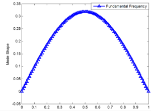
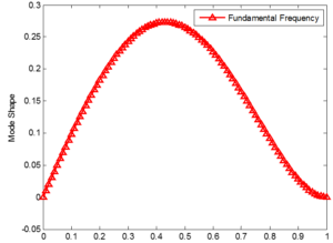
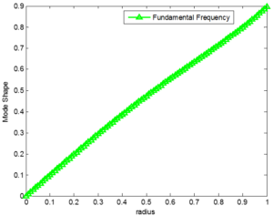
The solution of Laplace and Variation iteration method is presented here. Table 2 shows the comparison of present results to that of previously published work. It is realized from the Table 2 that, good agreements is achieved with that of the past results.The fundamental modal shape of the thin rectangular plate are shown in Figures 3, 4, 5 and it is observed that the shape obeys classical plate theory. Also, Table 3 shows different deflection values of transverse displacement for the first three mode frequency parameters of SC, SS and SF boundary condition considered. Table 4 shows the convergence study, it is observed that the fundamental natural frequency converges at the third iteration while higher modes are obtained by increasing the number of iterations. This phenomenon is peculiar to vibration problem.
Table 2. Showing validation of results.
Edge
Condition/Dimensionless
Simply-supported
(SS)
Simply supported
-Clamped (SC)
Simply-supported
-Free (SF)
Natural frequency
Bhat et al.[2]
Present
Leissa [38]
Present
Leissa [38]
Present
\(\Omega 1\)
19.7392
19.7434
23.6463
23.6486
11.7195
11.7606
3.1. Basic ideal of Laplace transform
If \(f(t)\) is a function of a variable \(t\). \(\mathscr{L}{F(t)}\) and is defined by the integral:3.2. Laplace and variation iteration method
Assuming the following nonlinear differential equation:3.3. Application of LVIM to the governing equation
Following the basic principle of LVIM , the governing equation is now analyzed as:Table 1. Parameters for validation of the model.
| Edge Condition/Dimensionless |
Simply-supported (SS) |
Simply supported -Clamped (SC) |
Simply-supported -Free (SF) |
|||
|---|---|---|---|---|---|---|
| Natural frequency | Bhat et al.;[2] | Present | Leissa [38] | Present | Leissa [38] | Present |
| \(\Omega 1\) | 19.7392 | 19.7434 | 23.6463 | 23.6486 | 11.7195 | 11.7606 |
4. Results and discussion
The solution of Laplace and Variation iteration method is presented here. Table 2 shows the comparison of present results to that of previously published work. It is realized from the Table 2 that, good agreements is achieved with that of the past results.The fundamental modal shape of the thin rectangular plate are shown in Figures 3, 4, 5 and it is observed that the shape obeys classical plate theory. Also, Table 3 shows different deflection values of transverse displacement for the first three mode frequency parameters of SC, SS and SF boundary condition considered. Table 4 shows the convergence study, it is observed that the fundamental natural frequency converges at the third iteration while higher modes are obtained by increasing the number of iterations. This phenomenon is peculiar to vibration problem.Table 2. Showing validation of results.
| Edge Condition/Dimensionless |
Simply-supported (SS) |
Simply supported -Clamped (SC) |
Simply-supported -Free (SF) |
|||
|---|---|---|---|---|---|---|
| Natural frequency | Bhat et al.[2] | Present | Leissa [38] | Present | Leissa [38] | Present |
| \(\Omega 1\) | 19.7392 | 19.7434 | 23.6463 | 23.6486 | 11.7195 | 11.7606 |
Figure 3. Fundamental mode shape of simply supported condition at both edges
Figure 4. Fundamental mode shape of simply supported with clamped edge condition
Figure 5. Fundamental mode shape of Simply Supported Condition at one edge and free at other edge
Table 3. Results of different deflection values.
| Transverse displacement | SF | SS | SC | SF | SS | SC | SF | SS | SC |
|---|---|---|---|---|---|---|---|---|---|
| \(\Omega 1\) | \(\Omega 2\) | \(\Omega 3\) | |||||||
| w[0] | 0.0000 | 0.0000 | 0.0000 | 0.0000 | 0.0000 | 0.0000 | 0.0000 | 0.0000 | 0.0000 |
| w[0.05] | 0.0500 | 0.0498 | 0.0497 | 0.0496 | 0.0492 | 0.0490 | 0.0489 | 0.0482 | 0.0479 |
| w[0.10] | 0.0998 | 0.0984 | 0.0978 | 0.0970 | 0.0935 | 0.0921 | 0.0916 | 0.0858 | 0.0837 |
| w[0.15] | 0.1492 | 0.1445 | 0.1425 | 0.1400 | 0.1288 | 0.1240 | 0.1224 | 0.1048 | 0.0983 |
| w[0.20] | 0.1981 | 0.1871 | 0.1825 | 0.1767 | 0.1514 | 0.1410 | 0.1376 | 0.1009 | 0.0881 |
| w[0.25] | 0.2464 | 0.2251 | 0.2163 | 0.2054 | 0.1592 | 0.1409 | 0.1351 | 0.0750 | 0.0556 |
| w[0.30] | 0.2938 | 0.2575 | 0.2429 | 0.2248 | 0.1514 | 0.1237 | 0.1153 | 0.0328 | 0.0091 |
| w[0.35] | 0.3403 | 0.2836 | 0.2615 | 0.2340 | 0.1288 | 0.0915 | 0.0807 | -0.0166 | -0.0397 |
| w[0.40] | 0.3857 | 0.3027 | 0.2715 | 0.2323 | 0.0935 | 0.0482 | 0.0358 | -0.0623 | -0.0784 |
| w[0.45] | 0.4300 | 0.3144 | 0.2727 | 0.2199 | 0.0492 | -0.0011 | -0.0134 | -0.0945 | -0.0973 |
| w[0.50] | 0.4732 | 0.3183 | 0.2652 | 0.1971 | 0.0000 | -0.0506 | -0.0607 | -0.1061 | -0.0915 |
| w[0.55] | 0.5153 | 0.3144 | 0.2496 | 0.1647 | -0.0492 | -0.0945 | -0.0998 | -0.0946 | -0.0624 |
| w[0.60] | 0.5564 | 0.3027 | 0.2266 | 0.1239 | -0.0935 | -0.1275 | -0.1254 | -0.0624 | -0.0173 |
| w[0.65] | 0.5967 | 0.2836 | 0.1976 | 0.0760 | -0.1288 | -0.1462 | -0.1340 | -0.0167 | 0.0326 |
| w[0.70] | 0.6363 | 0.2575 | 0.1641 | 0.0227 | -0.1514 | -0.1487 | -0.1240 | 0.0327 | 0.0751 |
| w[0.75] | 0.6757 | 0.2251 | 0.1279 | -0.0345 | -0.1592 | -0.1356 | -0.0958 | 0.0750 | 0.0999 |
| w[0.80] | 0.7154 | 0.1871 | 0.0914 | -0.0939 | -0.1514 | -0.1095 | -0.0520 | 0.1009 | 0.1018 |
| w[0.85] | 0.7561 | 0.1445 | 0.0571 | -0.1542 | -0.1288 | -0.0754 | 0.0036 | 0.1048 | 0.0821 |
| w[0.90] | 0.7987 | 0.0984 | 0.0281 | -0.2148 | -0.0935 | -0.0400 | 0.0664 | 0.0859 | 0.0487 |
| w[0.95] | 0.8444 | 0.0498 | 0.0078 | -0.2753 | -0.0492 | -0.0117 | 0.1325 | 0.0482 | 0.0155 |
| w[1.00] | 0.8948 | -9.0000 | -9.0000 | -0.3364 | 0.0000 | 0.0000 | 0.1995 | 0.0000 | 0.0000 |
Table 4. Showing convergence study of the results.
| Edge Condition /Dimensionless Natural frequency |
Iteration | (SS) | (SC) | ||||
|---|---|---|---|---|---|---|---|
| Bhat et al. [39] | Present | Leissa [38] | Present | Leissa [38] | Present | ||
| \(\Omega 1\) | N3 | 19.7392 | 19.7434 | 23.6463 | 23.6486 | 11.7195 | 11.7606 |
| \(\Omega 1\) | N4 | 19.7392 | 19.9574 | 23.6463 | 23.8905 | 11.7195 | 11.7445 |
| \(\Omega 2\) | 49.3481 | 49.3271 | 58.6465 | 58.6240 | 27.7563 | 27.7563 | |
| \(\Omega 1\) | N6 | 19.7392 | 19.7418 | 23.6463 | 23.6487 | 11.7195 | 11.6855 |
| \(\Omega 2\) | 49.3481 | 49.0637 | 58.6465 | 58.3220 | 27.7563 | 27.6965 | |
| \(\Omega 1\) | N7 | 19.7392 | 19.7394 | 23.6463 | 23.6465 | 11.7195 | 11.6846 |
| \(\Omega 2\) | 49.3481 | 49.3271 | 58.6465 | 58.6240 | 27.7563 | 27.7563 | |
4.1. Effect of foundation parameter on natural frequency
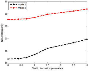
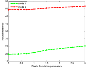
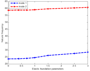
Table 5 illustrates the impact of foundation parameter on natural frequency. It is clear from the Figures 6, 7 and 8 that the foundation parameter has impact on natural frequency, increasing values of the foundation parameter increases the natural frequency. This satisfies the principle of classical vibration. Stiffness increment results to natural frequency increment. This also corroborated with finding reported in [38]. The effect of increase in natural frequency is much significant in higher values of the elastic foundation.Table 5.Variation elastic foundation coefficient on natural frequency.
| Edge Condition | Natural frequency | kw=5 | kw=15 | kw=45 | kw=120 | kw=200 | kw=250 |
|---|---|---|---|---|---|---|---|
| SS | \(\Omega 1\) | 19.865457 | 20.115575 | 20.847934 | 22.575127 | 24.282429 | 25.291033 |
| \(\Omega 2\) | 49.398659 | 49.49977 | 49.801882 | 50.549258 | 51.334467 | 51.81918 | |
| SC | \(\Omega 1\) | 23.751809 | 23.961395 | 24.579431 | 26.060476 | 27.552648 | 28.445534 |
| \(\Omega 2\) | 58.688978 | 58.774102 | 59.02877 | 59.660676 | 60.327409 | 60.7404 | |
| SF | \(\Omega 1\) | 11.896571 | 12.309687 | 13.473248 | 16.016504 | 18.34471 | 19.660326 |
| \(\Omega 2\) | 27.846269 | 28.025251 | 28.555467 | 29.839817 | 31.151479 | 31.94393 |
Figure 6. Variation of elastic foundation parameter on SF edge condition
Figure 7. Variation of elastic foundation parameter on SS-edge condition
Figure 8. Variation of elastic foundation parameter on SC-edge condition
4.2. Effect of variation of aspect ratio on natural frequency
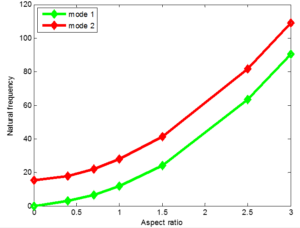
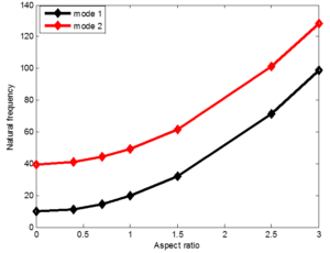
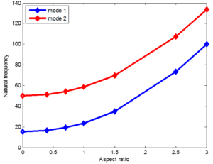
The influence of aspect ratio on natural frequency are shown in Table 6 and Figures 9, 10, 11 respectively. It is shown that, the natural frequency increase with increases in aspect ratio. This is because, the plate becomes more stiff as the aspect ratio increases resulting in the natural frequency increases.Figure 9. Variation of Aspect ratio on SF edge condition
Figure 10. Variation of Aspect ratio on SS edge condition
Figure 11. Variation of Aspect ratio on SC edge condition
Table 6. Variation of aspect ratio on natural frequency.
| Edge Condition | Natural frequency | \(\lambda=0.4\) | \(\lambda=0.7\) | \(\lambda=1.0\) | \(\lambda=1.5\) | \(\lambda=2.5\) | \(\lambda=3.0\) |
|---|---|---|---|---|---|---|---|
| SS | \(\Omega 1\) | 11.448741 | 14.705711 | 19.739209 | 32.076214 | 71.554632 | 98.696055 |
| \(\Omega 2\) | 41.057554 | 44.314525 | 49.348024 | 61.685024 | 101.16349 | 128.3048 | |
| SC | \(\Omega 1\) | 16.627624 | 19.277232 | 23.64632 | 35.051125 | 73.438926 | 100.26994 |
| \(\Omega 2\) | 51.326727 | 54.171092 | 58.646365 | 69.912813 | 107.42 | 133.79231 | |
| SF | \(\Omega 1\) | 3.0081474 | 6.562375 | 11.684537 | 24.010127 | 63.28683 | 90.296225 |
| \(\Omega 2\) | 17.636147 | 21.826148 | 27.756345 | 41.173975 | 81.606845 | 108.92412 |
5. Conclusion
In this study, the dynamic analysis of isotropic rectangular plates resting on Winkler and Pasternak foundations is analyzed. The governing equation is transform to nonlinear ordinary differential equation using Galerkin method of separation. The nonlinear ordinary differential equations have been solved using Laplace transform and variation of iteration method. The accuracies of the obtained analytical solutions were ascertained with the results obtained by earlier researcher. The obtained analytical solutions were used to examine the effects of foundation parameter, aspect ratio. The rate of convergence is increased with the introduction of exact method for analyzing the linear part of the governing equation while the remaining part are treated with variation of iteration method, practical applications of the study are base plate of tower, steel hinged steel column structures and culvert covers. From the parametric studies, the following observations were established:- Increase in elastic foundation parameter increases the natural frequency.
- Increase in aspect ratio increases the natural frequency.
- Increasing the combine elastic foundation parameters increases the natural frequency.
- Accurate higher mode frequency can be obtained with increase in number of iterations.
- SF boundary condition has the least value of frequency parameter followed by SS edge condition.
- The effect of increase in natural frequency is much significant in higher value of the elastic foundation.
Abbreviations
| Abbreviations | Nomenclature |
|---|---|
| \(a\) | Length of the plate |
| \(b\) | Width of the plate |
| \(C\) | Clamped edge plate |
| \(E\) | Young's modulus |
| \(F\) | Free edge support |
| \(S\) | Simply supported edge |
| \(d/dx\) | Differential operator |
| \(w\) | Dynamic deflection |
| \(X\) | space coordinate along the length of thin plate Symbol |
| \(h\) | plate thickness |
| \(\rho\) | Mass density |
| \(D\) | Modulus of elasticity |
| \(\Omega\) | natural frequency |
Acknowledgments
The author expresses sincere appreciation to the management of University of Lagos, Nigeria, for providing material supports and good environment for this work.Author Contributions
All authors contributed equally to the writing of this paper. All authors read and approved the final manuscript.Conflicts of Interest:
The authors declare no conflict of interest.References
- Jain, R. K., & Soni, S. R. (1973). Free vibrations of rectangular plates of parabolically varying thickness. Indian Journal of Pure and Applied Mathematics, 4(3), 267-277. [Google Scholor]
- Bhat, R. B. (1985). Natural frequencies of rectangular plates using characteristic orthogonal polynomials in Rayleigh-Ritz method. Journal of Sound and Vibration, 102(4), 493-499. [Google Scholor]
- Balkaya, M., Kaya, M. O., & Sağlamer, A. (2009). Analysis of the vibration of an elastic beam supported on elastic soil using the differential transform method. Archive of Applied Mechanics, 79(2), 135-146.[Google Scholor]
- Gupta, A. K., Saini, M., Singh, S., & Kumar, R. (2014). Forced vibrations of non-homogeneous rectangular plate of linearly varying thickness. Journal of Vibration and Control, 20(6), 876-884.[Google Scholor]
- Civalek, O., & Demir, C. (2011). Buckling and bending analyses of cantilever carbon nanotubes using the euler-bernoulli beam theory based on non-local continuum model. Asian Journal of Civil Engineering, 12(5), 651-661.[Google Scholor]
- AkgÖz, B., & Civalek, Ö. (2011). Buckling analysis of cantilever carbon nanotubes using the strain gradient elasticity and modified couple stress theories. Journal of Computational and Theoretical Nanoscience, 8(9), 1821-1827.[Google Scholor]
- Demir, C., Mercan, K., & Civalek, Ö. (2016). Determination of critical buckling loads of isotropic, FGM and laminated truncated conical panel. Composites Part B: Engineering, 94, 1-10.[Google Scholor]
- Zenkour, A. M. (2001). Buckling and free vibration of elastic plates using simple and mixed shear deformation theories. Acta mechanica, 146(3-4), 183-197.[Google Scholor]
- Mercan, K., & Civalek, Ö. (2017). Buckling analysis of Silicon carbide nanotubes (SiCNTs) with surface effect and nonlocal elasticity using the method of HDQ. Composites Part B: Engineering, 114, 34-45. [Google Scholor]
- Civalek, Ö., & Acar, M. H. (2007). Discrete singular convolution method for the analysis of Mindlin plates on elastic foundations. International Journal of Pressure Vessels and Piping, 84(9), 527-535.[Google Scholor]
- Baltacioglu, A. K., AkgÖz, B., & Civalek, Ö. (2010). Nonlinear static response of laminated composite plates by discrete singular convolution method. Composite structures, 93(1), 153-161.[Google Scholor]
- Zhong, H., & Yu, T. (2009). A weak form quadrature element method for plane elasticity problems. Applied Mathematical Modelling, 33(10), 3801-3814.[Google Scholor]
- Mercan, K., & Civalek, Ö. (2016). DSC method for buckling analysis of boron nitride nanotube (BNNT) surrounded by an elastic matrix. Composite structures, 143, 300-309.[Google Scholor]
- Duan, G., & Wang, X. (2014). Vibration analysis of stepped rectangular plates by the discrete singular convolution algorithm. International Journal of Mechanical Sciences, 82, 100-109.[Google Scholor]
- Zienkiewicz, O. C., & Taylor, R. L. (1989). The finite element method: basic formulation and linear problems (Vol. 1, pp. 1-20). London: McGraw-Hill.[Google Scholor]
- Reddy, J. N. (1993). An introduction to the finite element method. New York: McGraw-Hill.[Google Scholor]
- Yang, X. D., Zhang, W., Chen, L. Q., & Yao, M. H. (2012). Dynamical analysis of axially moving plate by finite difference method. Nonlinear Dynamics, 67(2), 997-1006. [Google Scholor]
- Numayr, K. S., Haddad, R. H., & Haddad, M. A. (2004). Free vibration of composite plates using the finite difference method. Thin-walled structures, 42(3), 399-414.[Google Scholor]
- Yeh, Y. L., Jang, M. J., & Wang, C. C. (2006). Analyzing the free vibrations of a plate using finite difference and differential transformation method. Applied mathematics and computation, 178(2), 493-501.[Google Scholor]
- Lezgy-Nazargah, M. (2016). A high-performance parametrized mixed finite element model for bending and vibration analyses of thick plates. Acta Mechanica, 227(12), 3429-3450.[Google Scholor]
- Civalek, Ö. (2017). Free vibration of carbon nanotubes reinforced (CNTR) and functionally graded shells and plates based on FSDT via discrete singular convolution method. Composites Part B: Engineering, 111, 45-59.[Google Scholor]
- Khuri, S. A., & Sayfy, A. (2012). A Laplace variational iteration strategy for the solution of differential equations. Applied Mathematics Letters, 25(12), 2298-2305.[Google Scholor]
- Meirovitch, L. (1980). Computational methods in structural dynamics (Vol. 5). Netherlands: Springer Science & Business Media.[Google Scholor]
- Wu, J. H., Liu, A. Q., & Chen, H. L. (2007). Exact solutions for free-vibration analysis of rectangular plates using Bessel functions. Journal of Applied Mechanics, 74(6), 1247-1251.[Google Scholor]
- Xing, Y., & Liu, B. (2009). New exact solutions for free vibrations of rectangular thin plates by symplectic dual method. Acta Mechanica Sinica, 25(2), 265. [Google Scholor]
- Xing, Y., & Liu, B. (2009). Closed form solutions for free vibrations of rectangular Mindlin plates. Acta Mechanica Sinica, 25(5), 689.[Google Scholor]
- Ozturk, B., Coskun, S. B., Koc, M. Z., & Atay, M. T. (2010). Homotopy perturbation method for free vibration analysis of beams on elastic foundation. In IOP Conference Series: Materials Science and Engineering (Vol. 10, No. 1, p. 012158). IOP Publishing.[Google Scholor]
- Njoku, K. O., Ezeh, J. C., Ibearugbulem, O. M., Ettu, L. O., & Anyaogu, L. (2013). Free vibration analysis of thin rectangular isotropic CCCC plate using Taylor series formulated shape function in Galerkin's method. Academic Research International, 4(4), 126.[Google Scholor]
- Pirbodaghi, T., Ahmadian, M. T., & Fesanghary, M. (2009). On the homotopy analysis method for non-linear vibration of beams. Mechanics Research Communications, 36(2), 143-148.[Google Scholor]
- He, J. H. (2003). Homotopy perturbation method: a new nonlinear analytical technique. Applied Mathematics and computation, 135(1), 73-79.[Google Scholor]
- He, J. H. (2004). The homotopy perturbation method for nonlinear oscillators with discontinuities. Applied mathematics and computation, 151(1), 287-292.[Google Scholor]
- He, J. H. (1998). Approximate solution of nonlinear differential equations with convolution product nonlinearities. Computer methods in applied mechanics and engineering, 167(1-2), 69-73.[Google Scholor]
- He, J. H. (2000). Variational iteration method for autonomous ordinary differential systems. Applied Mathematics and Computation, 114(2-3), 115-123.[Google Scholor]
- He, J. H. (1999). Variational iteration method--a kind of non-linear analytical technique: some examples International journal of non-linear mechanics, 34(4), 699-708.[Google Scholor]
- He, J. H. (2005). A generalized variational principle in micromorphic thermoelasticity. Mechanics Research Communications, 32(1), 93-98.[Google Scholor]
- He, J. H. (2006). Some asymptotic methods for strongly nonlinear equations. International journal of Modern physics B, 20(10), 1141-1199.[Google Scholor]
- Chakraverty, S. (2008). Vibration of plates. Boca Raton: CRC press.[Google Scholor]
- Leissa, A. W. (1973). The free vibration of rectangular plates. Journal of sound and vibration, 31(3), 257-293.[Google Scholor]


