Engineering and Applied Science Letter
ISSN: 2617-9709 (Online) 2617-9695 (Print)
DOI: 10.30538/psrp-easl2021.0066
Qualitative analysis of a mathematical model of divorce epidemic with anti-divorce therapy
Reuben Iortyer Gweryina\(^1\), Francis Shienbee Kaduna, Muhammadu Yahaya Kura
Department of Mathematics/Statistics/Computer Science, College of Science, Nigeria.; (R.I.G)
Federal University of Agriculture Makurdi, Makurdi, Nigeria.; (F.S.K)
Department of Mathematics/Statistics, Federal Polytechnic Nasarawa, Nigeria.; (M.Y.K)
Abstract
Keywords:
1. Introduction
Marriage is a socially accepted union or legal contract between two persons that established rights and obligations between them and their in-laws as well as the society. It can sometimes be referred to as the union of matrimony or wedlock, where interpersonal sexual relationship is biologically acknowledged [1]. The institution of marriage originally was meant to be a union of no bitterness. However, ugly experiences have emerged in which divorce and separation remain the most re-occurring decimals. The later phenomena are likely to happen when the ratio of negative to positive behaviour is equal or greater than unity. Divorce is the dissolution of marriage between two persons [2] which has a deformable mark on the family structure in our present era. This bitter trend continues to persist across Africa and the developed nations with no stigmatization. The immediate causes of divorce may not be limited to early marriage, less education, low income, premarital cohabitation and pregnancy, infidelity and lack of religion affiliation [3].
Divorce is an endemic issue that seriously affects the social and economic structure of contemporary society as much as any disease. Approximately one – half of all first marriages in the world end up in divorce or separation [4], with even higher rates of divorce for second marriages [5]. Separation leads to divorce as 75% of separation eventually result in divorce [6]. Divorce terms to increase childhood poverty and illiteracy rates [7]. It becomes important to eliminate this deadly social virus from our society.
Mathematical modelling has been used as a veritable tool for the control of epidemics in the past decades, and we can adopt it for the containment of the spread of divorce in marital institutions. In the past, concern has been focused on the influence of economy [8] and social contagion [9] on divorce models. Recently, [2] formulated a model for the spread of divorce in Ghana with three major compartments; Married, Divorced and Separated cases. Meanwhile, [10] extended their work to include the population of singles without any divorce prevention measure. Other mathematical studies on this subject matter can be found in [11,12,13]. Like other authors [2,9,10], we constructed a mathematical model for the spread of divorce epidemic. Apart from that, we incorporate a class of restored marital cases with anti-divorce therapy and reconciliation to the model of [10] using standard incidence function as the force of marital disunity, where the social family disorder is spread by divorced and separated persons over the married individuals. This is a major feature missing in the past works.
The organization of this paper is as follows: In Section 2, we formulate the model and establish the existence of equilibra and their local stability. In Section 3, we prove the global dynamics of each of the feasible steady states of the system (2) by constructing Lyapunov functions. In Section 4, we present the results and discussion of the numerical simulation. Finally, a brief conclusion is given in Section 5 to end this work.
2. Model construction
The present model derived its motivation from the work of [10], in which for the purpose of clarity, the basic model can be stated as;- People who are single or individuals who are ready for marriage but not yet married.
- Some Separated cases may resort to divorced but not vice-versa.
- Divorce or Separated cases restored can remain unbroken.
- Only Separated cannot be remarried.
- People who divorce can remarry or remain single.
- The anti-divorce parameter changes from 0 to 1 \((0\leq\phi\leq1)\).
Table 1. Variables and parameters of the model (2).
| <b>Variables</b> | <b>Description</b> |
|---|---|
| \(S_{1}(t)\) | Number of singles who are due for marriage at time \(t\) |
| \(M(t)\) | Number of Married cases at time \(t\) |
| \(D(t)\) | Number of Divorced cases at time \(t\) |
| \(S_{2}(t)\) | Number of Separated cases at time \(t\) |
| \(R(t)\) | Number of Restored Marital cases at time \(t\) |
| Parameters | Description |
| \(Q\) | Recruitment rate for the Single individuals |
| \(\beta_{1}\) | Divorced rate of the married |
| \(\beta_{2}\) | Separated rate of the married |
| \(\alpha_{1}\) | Rate of getting married by the singles |
| \(\alpha_{2}\) | Rate of re-marriage after divorced |
| \(d_{3}\) | Separated rate of the married |
| \(d_{2}\) | Proportion of married individuals that divorced |
| \(d_{1}\) | Proportion of married cases that results into Separation |
| \(r_{1}\) | Rate of restoring divorced cases in marriage by reconciliation |
| \(r_{2}\) | Rate of restoring Separated cases in marriage through reconciliation |
| \(\gamma\) | Rate of remaining single after divorce |
| \(\phi\) | Anti-divorce parameter \((0\leq\phi\leq1)\) |
| \(\mu\) | Natural death rate of individuals |
| \(\lambda_{m}\) | Force of marital disunity |
Note that, the first four Variables and the first seven Parameters in Table 1 have the same meaning as in model (1) [10]. However, \(\beta\) which is the rate of Separated getting married again in model (1) is disputed and so ignored in our study.
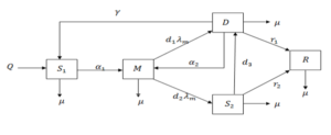
Figure 1. Model flow-diagram of divorce epidemic
From the model flow-diagram of divorce epidemic and assumptions, the following differential equations are derived;
2.1. Model steady states
At the steady state, the system (2) takes the form2.2. Divorce control reproduction number
The computation of the divorce controlled reproduction number denoted here by \(R_{ed} \) is done following the standard next generation matrix explained in [14] with the usual notation being given as; \[R_{ed}=\rho \left(F V^{-1}\right)=(1-\phi)\frac{\alpha_{1}}{\omega_{1}} \left(\frac{\beta_{1} (d_{1} \omega_{3}+ d_{2} d_{3})+\beta_{2} d_{2} \omega_{2}}{\omega_{2} \omega_{3}}\right),\] with \[F=(1-\phi)\frac{\alpha_{1}}{\omega_{1}}\begin{pmatrix} d_{1}\beta_{1} & d_{1}\beta_{2} \\ d_{2}\beta_{1} & d_{2}\beta_{2}\\ \end{pmatrix}\quad \text{and}\quad V^{-1}=\begin{pmatrix} \frac{1}{\omega_{2}} & \frac{d_{3}}{\omega_{2} \omega_{3}}\\ 0 & \frac{1}{\omega_{3}}\\ \end{pmatrix}.\] In the absence of anti-divorce therapy and reconciliation, \( \phi=0, r_{1}=r_{2}=0 \), we derive divorce reproduction number as; \[R_{d}=\frac{\alpha_{1}}{\omega_{1}} \left[\frac{\beta_{1} [d_{1} (\mu+d_{3})+d_{2} d_{3}]+\beta_{2} d_{2} (\mu+\gamma+\alpha_{2})}{(\mu+d_{3})(\mu+\gamma+\alpha_{2})}\right].\] However, for single intervention in terms of anti-divorce therapy and reconciliation only we have the respective reproduction numbers as; \begin{align*} R_{ad}&=(1-\phi)\frac{\alpha_{1}}{\omega_{1}} \left[\frac{\beta_{1}[d_{1} (\mu+d_{3})+d_{2} d_{3}]+\beta_{2} d_{2} (\mu+\gamma+\alpha_{2})}{(\mu+d_{3})(\mu+\gamma+\alpha_{2})}\right],\\ R_{ec}&=\frac{\alpha_{1}}{\omega_{1}} \left(\frac{\beta_{1} (d_{1} \omega_{3}+ d_{2} d_{3})+\beta_{2} d_{2} \omega_{2}}{\omega_{2} \omega_{3}}\right).\end{align*} Interestingly, it can be deduced from Theorem 2 in [14] that:Claim 1. The DFE is locally asymptotically stable in the case \( R_{ed}< 1\) and unstable when \( R_{ed}>1\).
2.3. Existence and local stability of divorce-endemic equilibrium
The existence of divorce endemic equilibrium follows immediately from (8) where \(\lambda_{m}^{**}\neq0\). Therefore, solving the remaining part of the equation leads toRecall from (10) that \(\lambda_{m}^{**}>0\) iff \(R_{ed}>1\) and \(\alpha_{1}>\alpha_{2}\), which are the necessary conditions for divorce to persist in marriage institution.
The method of linearization process of the system (2) at DE gives the following Jacobian Matrix
Claim 2. The divorce endemic equilibrium DE is locally asymptotically if \( R_{ed}>1\) and \(\frac{M^{**}}{N^{**}}< 1\).
3. Global dynamics
3.1. Global stability of DFE
This section discusses the global behavior of the model (2) at the divorce free equilibrium state following the well-known stability method of Lyapunov functions [16].Claim 3. The system (2) admits a globally asymptotically DFE iff \( R_{ed}< 1\).
Proof. By matrix theoretic approach as done in [16] we derive the following Lyapunov function \[L(t)=\frac{\beta_{1}}{\omega_{2}} D +\left(\frac{\beta_{i} d_{3}}{\omega_{2} \omega_{3}}+\frac{\beta_{2}}{\omega_{3}}\right) S_{2},\] whose time derivative is given by \begin{align*} L^{'}(t) =&\frac{\beta_{1}}{\omega_{2}}\left[d_{1} \left((1-\phi) \frac{\beta_{1} D + \beta_{2} S_{2}}{N}\right)M + d_{3} S_{2}-\omega_{2} D\right]\\ &+\left(\frac{\beta_{i} d_{3}}{\omega_{2} \omega_{3}}+\frac{\beta_{2}}{\omega_{3}}\right)\left[d_{2}\left((1-\phi) \frac{\beta_{1} D + \beta_{2} S_{2}}{N}\right)M -\omega_{3} S_{2}\right]. \end{align*} Collecting like terms and simplifying leads to \begin{align*} L^{'}(t) & =(\beta_{1} D + \beta_{2} S_{2})\left[(1-\phi) \left(\frac{\beta_{1} (d_{1} \omega_{3}+ d_{2} d_{3})+\beta_{2} d_{2} \omega_{2}}{\omega_{2} \omega_{3}}\right)\frac{M}{N}-1\right]. \end{align*} Recall that at divorce-free equilibrium we have \(\frac{M}{N}=\frac{M^{0}}{N^{0}}=\frac{\alpha_{1}}{\omega_{1}}\) and so \begin{align*} L^{'}(t) & =(\beta_{1} D + \beta_{2} S_{2})\left[(1-\phi)\frac{\alpha_{1}}{\omega_{1}} \left(\frac{\beta_{1} (d_{1} \omega_{3}+ d_{2} d_{3})+\beta_{2} d_{2} \omega_{2}}{\omega_{2} \omega_{3}}\right)-1\right]. \end{align*} Thus, \( L^{'}(t) =(\beta_{1} D + \beta_{2} S_{2})(R_{ed}-1), \), \(L^{'}(t)\leqslant0\) if \(R_{ed}\leqslant1\) and \( D=S_{2}=0\). Therefore, by Lyapunov's stability theory [15], the equilibrium point \(E^{0} \) is globally asymptotically stable.
3.2. Global stability of DE
Claim 4. The divorce-endemic equilibrium of the system (2) at \(\alpha_{2}=0\) is globally stable if \(R_{ed}>1\).
Proof. Taking the Lyapunov function \( W_{1}(t)\) as in [17]
The differential coefficient of \(W_{1} (t)\) in (15) with the substitution of model (2) at \( \alpha_{2}=0\) gives
Since \((S_{1},M, D, S_{2},R)\neq(S_{1}^{**},M^{**},D^{**},S_{2}^{**},R^{**})\), \(W_{1}^{'} (t)< 0\), \(W_{1}^{'} (t)=0\) if \(2-\frac{S_{2}}{S_{2}^{**}}=\frac{S_{2}^{**}}{S_{2}}\leqslant0\) and \(S_{1}=S_{1}^{**}, M=M^{**}, D=D^{**}, S_{2}=S_{2}^{**}, R=R^{**} \). Hence, DE is globally stable by Lyapunov's stability theory [15].
4. Results and discussions
To aid the understanding of the analyzed results, we performed the numerical simulation of the proposed model using MATLAB ode45 solver and the parameter values given in Table 2.
Table 2. Values of variables and parameters of the model (2) used for numerical simulations.
| <b>Initial Variables</b> | <b>Value</b> | <b>Source</b> |
|---|---|---|
| \(S_{1}(0)\) | 50 | Assumed |
| \(M(0)\) | 40 | Assumed |
| \(D(0)\) | 15 | Assumed |
| \(S_{2}(0)\) | 15 | Assumed |
| \(R(0)\) | 10 | Assumed |
| <b>Parameter</b> | <b>Value</b> | <b>Source</b> |
| \(Q\) | 2 | Assumed |
| \(\beta_{1}\) | 0.022 | \cite{j} |
| \(\beta_{2}\) | 0.031 | \cite{j} |
| \(\alpha_{1}\) | 0.101 | \cite{j} |
| \(\alpha_{2}\) | 0.061 | \cite{j} |
| \(d_{3}\) | 0.021 | \cite{j} |
| \(d_{2}\) | 0.7 | Assumed |
| \(d_{1}\) | 0.3 | Assumed |
| \(r_{1}\) | 0.1 | Assumed |
| \(r_{2}\) | 0.3 | Assumed |
| \(\gamma\) | 0.01 | Assumed |
| \(\phi\) | 0.2 | Assumed |
| \(\mu\) | 0.02 | Estimated |
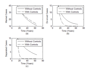
Figure 2. Impact of control measures (anti-divorce therapy and reconciliation) on (a) Married cases (b) Divorced cases (c) Separated cases using parameter values in Table 2.
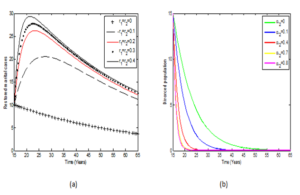
Figure 3. Impact of (a) reconciliation on Restored marital cases and (b) rate of remarriage on Divorced dynamics using parameter values in Table 2.
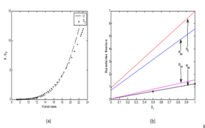
Figure 4. Relationship between (a) Married and the Divorced/Separated cases and (b) the reproduction numbers as a function of \( \beta_{1}\) using parameter values in Table 2.
In Figure 2(a), we observe that married couples develop the potentials to stay or remain in marriage longer when they attained marriage seminars/courses and exhibit the spirit of reconciliation in handling their differences. On the other hand, the union can easily break apart when the above mentioned controls are ignored.
The impact of anti-divorce control is depicted on the divorced cases in Figure 2(b). Here, the cases of marriage breaking apart (divorce) persist uniformly in the family circle where reconciliation and anti-divorce therapy are absent. Furthermore, the results supports that with the controls, divorced cases can be eliminated in marriage institutions and marriage couples who stay in marriage up to 30 years may have a stable family structure and no longer divorced their partners. This agrees with the result of high commission for planning of Morocco on marriage and divorce as contained in [11] which says that, couples with 20 years of experiences has a decreased divorce rate at 3%.
In the case of separated in Figure 2(c), the number rises higher for the scenario where the couples have not had proper premarital education and do not reconcile their misunderstanding on continuous bases. More so, the study reveals that marriage couples that live for over 15 years without separation are less venerable to divorce tendencies in marriage.
Figure 3(a) is a simple demonstration that increasing the rate of reconciliation impacts positively on the broken families by reuniting and hence increasing the number of restored cases. By implication, separated or divorced families will remain broken without adequate reconciliation process. Meanwhile, the effect of \( \alpha_{2}\) on the divorced is illustrated in Figure 3(b). The positive variation in \( \alpha_{2}\) reduces the cases of divorce in marriage. Therefore, it is recommendable to say that the re-marriage among the divorced helps to re-unite broken families.
The separated/divorced cases grow exponentially with respect to the married cases in Figure 4(a). This means that as long as married couples lived together, marital disorder in terms of separation or divorce may always be experienced among them. In other words, divorce cannot occur without marriage and the more marriage cases, the large scale of divorced population expected.
In Figure 4(b) we observed the behavioral trends of the model reproduction numbers that follows the inequality \(R_{ed}< R_{ec}< R_{ad}< R_{d}\). This symbolizes that the combination of reconciliation and anti-divorced protocols is beneficial in stabilizing marriages than when a single intervention is used. Furthermore, it is important to emphasize that, reconciliation in family settlement is better than marriage seminar/courses as proposed in [10]. This is also in line with the result of [19] that says; therapy is only a support but not a major component in solving marriage problems since \(R_{ec}< R_{ad} \). However, \(R_{d}\) standing above the rest of the reproduction ratios means that marriages without controls are fragile to crack or break apart in future.
5. Conclusion
A non-linear ordinary differential system of equations for examining the spread of divorce epidemic with anti-divorce therapy has been proposed and analyzed. Important results from the qualitative analysis of the modified model reveal that, the model has globally stable equilibrium states, namely the divorce-free and endemic equilibrium. Numerical results of this study suggest that the presence of correctional practices such as marriage seminar/courses and reconciliation efforts can ensure prolonged stable marriages and prevents cracks and repairs the breaking points (separation or divorce) in family structure. In addition, the marriage couples that escape separations in early 15 years of marriage and stay together in the next 15 years cannot divorce any longer.Author Contribution: All authors contributed equally to the writing of this paper. All authors read and approved the final manuscript.
Conflicts of Interest: The authors declare no conflict of interest.
References
- Wimalasena, N. A. (2016). An analytical study of definitions of the term ''marriage''. International Journal of Humanities and Social Science, 6(1), 166-174. [Google Scholor]
- Gambrah, P. P., & Adzadu, Y. (2018). Mathematical model of divorce epidemic in Ghana. International Journal of Statistics and Applied Mathematics, 3(2), 395-401. [Google Scholor]
- Mekonnen, Y., Kassa, K., & Ayalew, M. (2019). Prevalence, causes and consequences of divorce in Bahir Dar city, Ethiopia. African Journal of Social Work, 9(1), 3-78. [Google Scholor]
- Bramlett, M. D., & Mosher, W. D. (2002). Cohabitation, marriage, divorce, and remarriage in the United States. Division of Vital Statistics Series, 23(22), 32pp. [Google Scholor]
- Cherlin, A. (2009). Marriage, divorce, remarriage. Harvard University Press. [Google Scholor]
- Hawkins, A. J., Willoughby, B. J., & Doherty, W. J. (2012). Reasons for divorce and openness to marital reconciliation. Journal of Divorce & Remarriage, 53(6), 453-463. [Google Scholor]
- Anderson, J. (2014). The impact of family structure on the health of children: Effects of divorce. The Linacre Quarterly, 81(4), 378-387. [Google Scholor]
- Huang, J. T. (2003). Unemployment and family behavior in Taiwan. Journal of Family and Economic Issues, 24(1), 27-48. [Google Scholor]
- Duato, R., & Jódar, L. (2013). Mathematical modeling of the spread of divorce in Spain. Mathematical and Computer Modelling, 57(7-8), 1732-1737.[Google Scholor]
- Gambrah, P. P., & Adzadu, Y. (2018). Mathematical model of divorce epidemic in Ghana. International Journal of Statistics and Applied Mathematics, 3(2), 395-401. [Google Scholor]
- Lhous, M., Rachik, M., Laarabi, H., & Abdelhak, A. (2017). Discrete mathematical modeling and optimal control of the marital status: the monogamous marriage case. Advances in Difference Equations, 2017, Article No. 339, DOI: 10.1188/S13662-017-1390-0. [Google Scholor]
- Shah, J. N. H.,Pandya, P. M., & Satia, M. H. (2019). Global stability for Divorce in Arrange/Hove marriage due to extra marital affairs. International Journal of Scientific and Technology Research, Corpus ID: 203995063. [Google Scholor]
- Bruze, G., Svarer, M., & Weiss, Y. (2015). The dynamics of marriage and divorce. Journal of Labor Economics, 33(1), 123-170. [Google Scholor]
- Van den Driessche, P., & Watmough, J. (2002). Reproduction numbers and sub-threshold endemic equilibria for compartmental models of disease transmission. Mathematical biosciences, 180(1-2), 29-48. [Google Scholor]
- Martcheva, M. (2015). An introduction to mathematical epidemiology (Vol. 61). New York: Springer.[Google Scholor]
- Nwafor, E. U., Okoro, C. J., Inyama, S. C., Omame, A., & Mbachu, H. I. Analysis of a Mathematical Vaccination Model of an Infectious Measles Disease. FUTO Journal Series, 5(1), 168 - 188. [Google Scholor]
- Mpande, L. C., Kajunguri, D., & Mpolya, E. A. (2015). Modeling and stability analysis for measles metapopulation model with vaccination. Applied and Computational Mathematics, 4(6), 431-444. [Google Scholor]
- McCluskey, C. C. (2015). Using Lyapunov functions to construct Lyapunov functionals for delay differential equations. SIAM Journal on Applied Dynamical Systems, 14(1), 1-24. [Google Scholor]
- Plauche, H. P. (2014). The Hard Decisions: A Qualitative Study of Marital Reconciliation. Ph.D Thesis submitted to the Graduate Faculty of the Louisiana State University and Agriculture and Mechanical College, (2014), 129pp. [Google Scholor]


