Open Journal of Discrete Applied Mathematics
ISSN: 2617-9687 (Online) 2617-9679 (Print)
DOI: 10.30538/psrp-odam2019.0010
Analysis of the qualitative behaviour of an eighth-order fractional difference equation
Department of Mathematics, Faculty of Science, Taibah University, P.O. Box 30002, Saudi Arabia.; (M.B.A)
Department of Mathematics, College of Duba, University of Tabuk, P.O. Box 71491, Saudia Arabia.; (M.M.A)
\(^{1}\)Corresponding Author: mmutrafi@taibahu.edu.sa
Abstract
Keywords:
1. Introduction
ost fractional difference equations are studied from their qualitative behaviours of the governing equations. This can be strongly attributed to the fact that obtaining theexact solutions of these equations is quite sophisticated sometimes. A considerable number of authors has established the equilibria, stability, periodic solutions and boundedness of some nonlinear recursive relations. For example, Abdelrahman et al. [1] examined the asymptotic stability of the solutions of the following recursive equation \begin{equation*} x_{n+1}=ax_{n-l}+bx_{n-k}+f(x_{n-l},x_{n-k}). \end{equation*} Almatrafi et al. [2] investigated the qualitative behaviour of the following fourth-order rational difference equations \begin{equation*} x_{n+1}=\frac{\alpha x_{n}x_{n-3}}{\pm \beta x_{n-3} \pm \gamma x_{n-2}}. \end{equation*} El-Moneam et al. [3] introduced some results on the qualitative behaviour of the following recursive equation \[ x_{n+1}=Ax_{n}+Bx_{n-k}+Cx_{n-l}+Dx_{n-\sigma }+\frac{bx_{n-k}+hx_{n-l}}{% dx_{n-k}+ex_{n-l}}. \] Garić-Demirović et al. [4] presented the periodic solution and the stability character of the following second-order relation \begin{equation*} x_{n+1}=\dfrac{Ax_{n}^{2}+Bx_{n}x_{n-1}+Cx_{n-1}^{2}}{% ax_{n}^{2}+bx_{n}x_{n-1}+cx_{n-1}^{2}}. \end{equation*} In [5], the authors concerned with showing an analytical investigation about the following sixth-order difference equation \begin{equation*} x_{n+1}=\frac{Cx_{n-5}}{A+Bx_{n-2}x_{n-5}}. \end{equation*} Moreover, Khaliq and Hassan [6] examined the dynamic behaviour of the recursive equation given on the form \begin{equation*} x_{n+1}=ax_{n}+\frac{\alpha+\beta x_{n-k}}{A+Bx_{n-k}}. \end{equation*} Elabbasy et al. [7] studied the periodic solution, local stability, global attractivity and the solution of a special case from the equation given by \begin{equation*} x_{n+1}=ax_{n}-\frac{bx_{n}}{cx_{n}-dx_{n-1}}. \end{equation*} For more information about the dynamic behaviours of some fractional recursive equations, one can see [8, 9, 10, 11, 12, 13, 14, 15].Our main purpose in this paper is to investigate some qualitative behaviours such as the local stability, global stability and the periodicity of the following rational recursive equation
2. Analysis of Local Stability
In this section, we will examine the behaviour of the solutions around the equilibrium point and show that the solutions which start nearby the fixed point stay nearby the fixed point under a specific condition. The equilibrium point of Equation (1) is given by the following equation: \begin{equation*} \overline{x}=c_{1}\overline{x}+\frac{c_{2}\overline{x}}{c_{3}\overline{x}-c_{4}\overline{x}}, \end{equation*} which leads to \begin{equation*} \overline{x}=\frac{c_{2}}{\left( 1-c_{1}\right) \left( c_{3}-c_{4}\right) },\ c_{1} \neq 1, c_{3} \neq c_{4}. \end{equation*} Suppose that a function \(h:\left( 0,\infty \right)^{2}\longrightarrow \left( 0,\infty \right) \) is defined as followingTheorem 1. Let \(\left\vert c_{1}c_{3}-c_{4}\right\vert +c_{4}\left\vert 1-c_{1}\right\vert < \left\vert c_{3}-c_{4}\right\vert .\) Then, the fixed point of Equation (1) is locally asymptotically stable.
Proof. It can be simply observed from Theorem A of [16] that the equilibrium point of Equation (1) is locally asymptotically stable if \begin{equation*} \left\vert p_{1}\right\vert +\left\vert p_{2}\right\vert < 1. \end{equation*} This gives us \begin{equation*} \left\vert -\Bigg(c_{1}-\frac{c_{4}(1-c_{1})}{c_{3}-c_{4}}\Bigg)\right\vert +\left\vert -\frac{c_{4}(1-c_{1})}{c_{3}-c_{4}}\right\vert < 1, \end{equation*} which can be written on the following form \begin{equation*} \left\vert c_{1}(c_{3}-c_{4})-c_{4}(1-c_{1})\right\vert +c_{4}\left\vert 1-c_{1}\right\vert < \left\vert (c_{3}-c_{4})\right\vert . \end{equation*} Hence, \begin{equation*} \left\vert c_{1}c_{3}-c_{4}\right\vert +c_{4}\left\vert 1-c_{1}\right\vert < \left\vert c_{3}-c_{4}\right\vert . \end{equation*} This complete the proof.
3. Analysis of Global Stability
We now turn to introduce an appropriate condition under which the fixed point of Equation (1) is a global attractor.Theorem 2. \label{first glo. thm} Let \(c_{1}< \frac{c_{2}c_{4}s}{(c_{3}r-c_{4}s)^{2}},\) then the equilibrium point of Equation (1) is a global attractor if \(c_{1}c_{3}>c_{4}.\)
Proof. Let \(a,\ b \in \mathbb{R}\) and suppose that \(h:\left[ a,b\right] ^{2}\longrightarrow \left[ a,b\right] \) is a function defined by Equation (2). We assume that \(c_{1}< \frac{c_{2}c_{4}s}{(c_{3}r-c_{4}s)^{2}},\) then the function \(h\) is decreasing in \(r\) and increasing in \(s.\) Now, we suppose that \((\phi, \psi)\) is a solution to the system given by $$\phi=h(\psi,\phi),\ \psi=h(\phi,\psi).$$ Therefore, \begin{align*} \phi &= h(\psi,\phi)=c_{1} \psi +\frac{c_{2} \psi}{c_{3}\psi-c_{4}\phi}, \\ \psi&=h(\phi,\psi)=c_{1}\phi+\frac{c_{2}\phi}{c_{3}\phi-c_{4}\psi}. \end{align*} Clearing the denominators gives
Theorem 3. Let \(c_{1}>\frac{c_{2}c_{4}s}{(c_{3}r-c_{4}s)^{2}},\) then the equilibrium point of Equation (1) is a global attractor if \(c_{3}< c_{4}\) and \(c_{1}< 1.\)
Proof. The proof can be accomplished in a similar way to the previous one. Thus, it is omitted.
4. Periodicity of the solution
Equation (1) has no prime period two solutions. This property will be proved in the following theorem.%please rewrite this line to make it more clearTheorem 4. The Equation (1) has no prime period two solutions.
Proof. Assume that the Equation (1) has a prime period two solution given as follows \begin{equation*} \ldots,\ t,\ \tau,\ t,\ \tau,\ \ldots, \end{equation*} with \(t \neq \tau.\) From Equation (1), one can observe that \begin{eqnarray*} t&=&c_{1}t+\frac{c_{2}t}{c_{3}t-c_{4}t},\\ \tau &=& c_{1}\tau+\frac{c_{2}\tau}{c_{3}\tau-c_{4}\tau}. \end{eqnarray*} Hence, \begin{eqnarray*} (1-c_{1})t&=&\frac{c_{2}}{c_{3}-c_{4}},\\ (1-c_{1})\tau &=& \frac{c_{2}}{c_{3}-c_{4}}. \end{eqnarray*} This implies that \(t=\tau,\) which contradicts our assumption.
5. Special case of Equation (1)
This section is devoted to present the exact solution of the following recursive equationTheorem 5. Let \(\left \{x_{n}\right\}_{n=-7}^{\infty}\) be a solution of Equation (7) and assume that \(x_{-7}=\alpha,\ x_{-6}=\beta,\ x_{-5}=\gamma,\ x_{-4}=\delta,\ x_{-3}=\epsilon,\ x_{-2}=\zeta,\ x_{-1}=\kappa,\ x_{0}=\omega.\) Then, for \(n=0,1,2,...,\) the solution of Equation (7) is given by the following relations \begin{eqnarray*} x_{8n-7} &=&-\frac{\left[ \left( n-1\right) \alpha -n\epsilon \right] \left[ \alpha -\epsilon -n\right] }{\alpha -\epsilon },\ \ \ x_{8n-6}=-\frac{\left[ \left( n-1\right) \beta -n\zeta \right] \left[ \beta -\zeta -n\right] }{% \beta -\zeta }, \\ x_{8n-5} &=&-\frac{\left[ \left( n-1\right) \gamma -n\kappa \right] \left[ \gamma -\kappa -n\right] }{\gamma -\kappa },\ \ \ x_{8n-4}=-\frac{\left[ \left( n-1\right) \delta -n\omega \right] \left[ \delta -\omega -n\right] }{% \delta -\omega }, \\ x_{8n-3} &=&-\frac{\left[ n\alpha -\left( n+1\right) \epsilon \right] \left[ \alpha -\epsilon -n\right] }{\alpha -\epsilon },\ \ \ x_{8n-2}=-\frac{\left[ n\beta -\left( n+1\right) \zeta \right] \left[ \beta -\zeta -n\right] }{% \beta -\zeta }, \\ x_{8n-1} &=&-\frac{\left[ n\gamma -\left( n+1\right) \kappa \right] \left[ \gamma -\kappa -n\right] }{\gamma -\kappa },\ \ \ x_{8n}=-\frac{\left[ n\delta -\left( n+1\right) \omega \right] \left[ \delta -\omega -n\right] }{% \delta -\omega }. \end{eqnarray*}
Proof. It can be easily seen that the formulae are true at \(n=0.\) Next, we assume that \(n>0\) and suppose that our solution is correct at \(n-1\) as follows \begin{eqnarray*} x_{8n-15} &=&-\frac{\left[ \left( n-2\right) \alpha -\left( n-1\right) \epsilon \right] \left[ \alpha -\epsilon -n+1\right] }{\alpha -\epsilon },\ \ \ x_{8n-14}=-\frac{\left[ \left( n-2\right) \beta -\left( n-1\right) \zeta % \right] \left[ \beta -\zeta -n+1\right] }{\beta -\zeta }, \\ x_{8n-13} &=&-\frac{\left[ \left( n-2\right) \gamma -\left( n-1\right) \kappa \right] \left[ \gamma -\kappa -n+1\right] }{\gamma -\kappa },\ \ \ x_{8n-12}=-\frac{\left[ \left( n-2\right) \delta -\left( n-1\right) \omega % \right] \left[ \delta -\omega -n+1\right] }{\delta -\omega }, \\ x_{8n-11} &=&-\frac{\left[ \left( n-1\right) \alpha -n\epsilon \right] \left[ \alpha -\epsilon -n+1\right] }{\alpha -\epsilon },\ \ \ x_{8n-10}=-\frac{% \left[ \left( n-1\right) \beta -n\zeta \right] \left[ \beta -\zeta -n+1% \right] }{\beta -\zeta }, \\ x_{8n-9} &=&-\frac{\left[ \left( n-1\right) \gamma -n\kappa \right] \left[ \gamma -\kappa -n+1\right] }{\gamma -\kappa },\ \ \ x_{8n-8}=-\frac{\left[ \left( n-1\right) \delta -n\omega \right] \left[ \delta -\omega -n+1\right] }{\delta -\omega }. \end{eqnarray*} Now, we prove the first relation. Equation (7) gives \begin{eqnarray*} x_{8n-7} &=&x_{8n-11}+\frac{x_{8n-11}}{x_{8n-11}-x_{8n-15}} \end{eqnarray*} \begin{eqnarray*} &=&-\frac{\left[ \left( n-1\right) \alpha -n\epsilon \right] \left[ \alpha -\epsilon -n+1\right] }{\alpha -\epsilon }+\frac{-\frac{\left[ \left( n-1\right) \alpha -n\epsilon \right] \left[ \alpha -\epsilon -n+1\right] }{% \alpha -\epsilon }}{-\frac{\left[ \left( n-1\right) \alpha -n\epsilon \right] \left[ \alpha -\epsilon -n+1\right] }{\alpha -\epsilon }+\frac{\left[ \left( n-2\right) \alpha -\left( n-1\right) \epsilon \right] \left[ \alpha -\epsilon -n+1\right] }{\alpha -\epsilon }} \\ &=&-\frac{\left[ \left( n-1\right) \alpha -n\epsilon \right] \left[ \alpha -\epsilon -n+1\right] }{\alpha -\epsilon }-\frac{\left[ \left( n-1\right) \alpha -n\epsilon \right] }{\epsilon -\alpha } \\ &=&-\left[ \frac{\left[ \left( n-1\right) \alpha -n\epsilon \right] \left[ \alpha -\epsilon -n+1\right] }{\alpha -\epsilon }-\frac{\left[ \left( n-1\right) \alpha -n\epsilon \right] }{\alpha -\epsilon }\right] \\ &=&-\frac{\left[ \left( n-1\right) \alpha -n\epsilon \right] \left[ \alpha -\epsilon -n\right] }{\alpha -\epsilon }. \end{eqnarray*} We now prove the second formula. Again, Equation (7) gives \begin{eqnarray*} x_{8n-6} &=&x_{8n-10}+\frac{x_{8n-10}}{x_{8n-10}-x_{8n-14}} \\ &=&-\frac{\left[ \left( n-1\right) \beta -n\zeta \right] \left[ \beta -\zeta -n+1\right] }{\beta -\zeta }+\frac{-\frac{\left[ \left( n-1\right) \beta -n\zeta \right] \left[ \beta -\zeta -n+1\right] }{\beta -\zeta }}{-\frac{% \left[ \left( n-1\right) \beta -n\zeta \right] \left[ \beta -\zeta -n+1% \right] }{\beta -\zeta }+\frac{\left[ \left( n-2\right) \beta -\left( n-1\right) \zeta \right] \left[ \beta -\zeta -n+1\right] }{\beta -\zeta }} \\ &=&-\left[ \frac{\left[ \left( n-1\right) \beta -n\zeta \right] \left[ \beta -\zeta -n+1\right] }{\beta -\zeta }-\frac{\left[ \left( n-1\right) \beta -n\zeta \right] }{\beta -\zeta }\right] \\ &=&-\frac{\left[ \left( n-1\right) \beta -n\zeta \right] \left[ \beta -\zeta -n\right] }{\beta -\zeta }. \end{eqnarray*} The proofs of the remaining relations can be achieved in a similar way. Thus, the remaining proofs are omitted.
6. Numerical examples
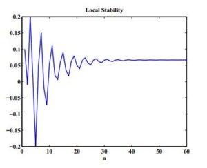
This section will confirm the above-mentioned theoretical analysis by providing some numerical examples.Example 1. In this example, we confirm the local stability of the equilibrium point under the values \(c_{1}=0.5,\ c_{2}=0.3,\ c_{3}=10,\ c_{4}=1,\ x_{-7}=-0.02,\ x_{-6}=0.15,\ x_{-5}=0.05,\ x_{-4}=-0.2,\ x_{-3}=0.01,\ x_{-2}=0.2,\ x_{-1}=-0.01,\ x_{0}=0.1. \) See Figure 1.
Figure 1. Local Stability of The Equilibrium Point.
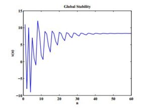
Example 2. Figure 2 shows the global stability of the fixed point when we let \(c_{1}=0.5,\ c_{2}=10,\ c_{3}=3,\ c_{4}=0.6,\ x_{-7}=12,\ x_{-6}=-1,\ x_{-5}=1,\ x_{-4}=7,\ x_{-3}=-9,\ x_{-2}=10,\ x_{-1}=-8,\ x_{0}=11. \)
Figure 2. Global Stability of The Equilibrium Point.
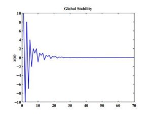
Example 3. In Figure 3, we plot the global stability under the conditions given in Theorem 3. Here, we consider the values \(c_{1}=0.5,\ c_{2}=0.025,\ c_{3}=5,\ c_{4}=6,\ x_{-7}=1,\ x_{-6}=2,\ x_{-5}=-2,\ x_{-4}=4,\ x_{-3}=-7,\ x_{-2}=8,\ x_{-1}=-10,\ x_{0}=10. \)
Figure 3. Global Stability of The Equilibrium Point.
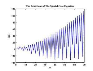
Example 4. The behaviour of the solution of Equation (7) is plotted in Figure 4 according to the following values: \(c_{1}=0.5,\ c_{2}=0.025,\ c_{3}=5,\ c_{4}=6,\ x_{-7}=1,\ x_{-6}=2,\ x_{-5}=-2,\ x_{-4}=4,\ x_{-3}=-7,\ x_{-2}=8,\ x_{-1}=-10,\ x_{0}=10.\)
Figure 4. Solution of The Special Case Equation.
7. Conclusion
This paper investigated the qualitative behaviour of Equation (1) and shown some numerical examples for these properties. For instance, Theorem 1 presents the condition under which the fixed point of Equation (1) is locally asymptotically stable. Moreover, Theorem 2 provides a simple condition under which the equilibrium point is a global attractor, while Theorem 3 proves the global stability if \(c_{3}< c_{4}\) and \(c_{1}< 1,\) hold. In Section 4, it has been proved that Equation (1) has no a prime period two solution. Theorem 5 introduces the exact solution of the Equation (7). Finally, Section 6 has been added to confirm all analytical work discussed in the previous sections.Competing Interests
The authors declare that they have no competing interests.References
- Abdelrahman, M. A. E., Chatzarakis, G. E., Tongxing, L., & Moaaz, O. (2018). On the difference equation \(x_{n+1}=ax_{n-l}+bx_{n-k}+f(x_{n-l},x_{n-k}).\) Advances in Difference Equations, 2018(1), 1-14.[Google Scholor]
- Almatrafi, M. B., Elsayed, E. M., & Alzahrani, F. (2018). Qualitative behavior of two rational difference equations. Fundamental Journal of Mathematics and Applications, 1(2), 194-204.[Google Scholor]
- El-Moneam, M. A., & Zayed, E. M. E. (2014). Dynamics of the rational difference equation. Information Sciences Letters, 3(2), 45-53.[Google Scholor]
- Garić-Demirović, M., Nurkanović, M., & Nurkanović, Z. (2017), Stability, periodicity and Neimark-Sacker bifurcation of certain homogeneous fractional difference equations. International Journal of Difference Equations, 12(1), 27-53.[Google Scholor]
- Ghazel, M., Elsayed, E. M., Matouk, A. E., & Mousallam, A. M. (2017). Investigating dynamical behaviors of the difference dquation \(x_{n+1}=Cx_{n-5}/(A+Bx_{n-2}x_{n-5})\). Journal of Nonlinear Sciences and Applications, 10, 4662-4679.
- Khaliq, A., & Hassan, S. S. (2018). Dynamics of a rational difference equation \(x_{n+1}=ax_{n}+(\alpha+\beta x_{n-k})/(A+Bx_{n-k}).\) International Journal of Advances in Mathematics, 2018(1), 159-179.
- Elabbasy, E. M., El-Metwally, H., & Elsayed, E. M. (2006). On the difference equation \(x_{n+1}=ax_{n}-(bx_{n})/(cx_{n}-dx_{n-1})\). Advances in difference Equations, 2006(1), 1-10. [Google Scholor]
- Almatrafi, M. B., Elsayed, E. M. (2018). Solutions and formulae for some systems of difference equations. MathLAB Journal, 1(3), 356-369.[Google Scholor]
- Almatrafi, M. B., Elsayed, E. M., & Alzahrani, F. (2019). Qualitative behavior of a quadratic second-order rational difference equation. International Journal of Advances in Mathematics, 2019(1), 1-14.[Google Scholor]
- Belhannache, F., Touafek, N., & Abo-zeid, R. (2016). On a higher-order rational difference equation. Journal of Applied Mathematics & Informatics, 34(5-6),369-382.[Google Scholor]
- Kostrov, Y., & Kudlak, Z. (2016). On a second-order rational difference equation with a quadratic term. International Journal of Difference Equations, 11(2), 179-202.[Google Scholor]
- Liu, K., Li, P., Han, F., & Zhong, W. (2018). Global dynamics of nonlinear difference equation \(x_{n+1}=A+x_{n}/x_{n-1}x_{n-2}\). Journal of Computational Analysis and Applications, 24(6), 1125-1132.[Google Scholor]
- Moranjkić, S., & Nurkanović, Z. (2017). Local and global dynamics of certain second-order rational difference equations containing quadratic terms. Advances in Dynamical Systems and Applications, 12(2), 123-157.[Google Scholor]
- Saleh, M. & Aloqeili, M. (2005). On the rational difference equation \(y_{n+1}=A+\frac{y_{n-k}}{y_{n}}\). Applied Mathematics and Computation, 171(1), 862-869. [Google Scholor]
- Saleh, M., & Farhat, A. (2017). Global asymptotic stability of the higher order equation \(x_{n+1}=\frac{ax_{n}+bx_{n-k}}{A+Bx_{n-k}}\). Journal of Applied Mathematics and Computing, 55(1-2), 135-148.[Google Scholor]
- Elabbasy, E. M., El-Metawally, H., & Elsayed, E. M. (2008). On the difference equation \(x_{n+1}=(ax_{n}^{2}+bx_{n-1}x_{n-k})/(cx_{n}^{2}+dx_{n-1}x_{n-k})\). Sarajevo Journal of Mathematics, 4(17), 1-10. [Google Scholor]
- Elsayed, E. M., & Alghamdi, A. (2016). Dynamics and global stability of higher order nonlinear difference equation. Journal of Computational Analysis and Applications, 21(3), 493-503. [Google Scholor]


