Open Journal of Discrete Applied Mathematics
ISSN: 2617-9687 (Online) 2617-9679 (Print)
DOI: 10.30538/psrp-odam2020.0035
Numerical analysis of least squares and perceptron learning for classification problems
Larisa Beilina
Department of Mathematical Sciences, Chalmers University of Technology and University of Gothenburg, SE-42196 Gothenburg, Sweden.;
larisa@chalmers.se
Abstract
Keywords:
1. Introduction
Machine learning is a field of artificial intelligence which gives computer systems the ability to ''learn'' using available data. Recently machine learning algorithms become very popular for analyzing of data and make prediction [1,2,3,4]. Linear models for classification is a part of supervised learning [1]. Supervised learning is machine learning task of learning a function which transforms an input to an output data using available input-output data. In supervised learning, every example is a pair consisting of an input object (typically a vector) and a desired output value (also called the supervisory signal). A supervised learning algorithm analyzes the training data and produces an inferred function, which can be used then for analyzing of new examples. Supervised Machine Learning algorithms include linear and logistic regression, multi-class classification, decision trees and support vector machines. In this work we will concentrate attention on study the linear and logistic regression algorithms. Supervised learning problems are further divided into Regression and Classification problems. Both problems have as goal the construction of a model which can predict the value of the dependent attribute from the attribute variables. The difference between these two problems is the fact that the attribute is numerical for regression and logical (belonging to class or not) for classification.
In this work are studied linear and polynomial classifiers, more precisely, the regularized versions of least squares and perceptron learning algorithms. The WINNOW algorithm for classification is also presented since it is used in numerical examples of Section 6 for comparison of different classification strategies. The classification problem is formulated as a regularized minimization problem for finding optimal weights in the model function. To formulate iterative gradient-based classification algorithms the Fréchet derivatives for the non-regularized and regularized least squares algorithms are presented. The Fréchet derivative for the perceptron algorithm is also rigorously derived.
Adding the regularization term in the functional leads to the optimal choice of weights such that they make a trade-off between observed data and obtaining a minimum of this functional. Different rules are used for choosing the regularization parameter in machine learning, and most popular are early stopping algorithm, bagging and dropout techniques [5], genetic algorithms [6], particle swarm optimization [7,8], racing algorithms [9] and Bayesian optimization techniques [10,11]. In this work are presented the most popular a priori and a posteriori Tikhonov's regularization rules for choosing the regularization parameter in the cost functional. Finally, performance of non-regularized versions of all classification algorithms with respect to applicability, reliability and efficiency is analyzed on simulated and experimental data sets [12,13].
The outline of the paper is as follows. In Section 2 are briefly formulated non-regularized and regularized classification problems. Least squares for classification are discussed in Section 3. Machine learning linear and polynomial classifiers are presented in Section 4. Tikhonov's methods of regularization for classification problems are discussed in Section 5. Finally, numerical tests are presented in Section 6.
2. Classification problem
The goal of regression is to predict the value of one or more continuous target variables \(t=\{t_i\}, i=1,...,m\) by knowing the values of input vector \(x=\{x_i\}, i=1,...,m\). Usually, classification algorithms are working well for linearly separable data sets.
Definition 1. Let \(A\) and \(B\) are two data sets of points in an \(n\)-dimensional Euclidean space. Then \(A\) and \(B\) are linearly separable if there exist \(n + 1\) real numbers \(\omega_1, ..., \omega_n, l\) such that every point \(x \in A\) satisfies \(\sum _{i=1}^{n}\omega_{i} x_{i} > l\) and every point \(x \in B\) satisfies \(\sum _{i=1}^{n}\omega_{i} x_{i} < -l\).
The classification problem is formulated as follows:
- Suppose that we have data points \(\{x_i\}, i=1,...,m\) which are separated into two classes \(A\) and \(B\). Assume that these classes are linearly separable.
- Our goal is to find the decision line which will separate these two classes. This line will also predict in which class will the new point fall.
In the non-regularized classification problem the goal is to find optimal weights \(\omega=(\omega_1,...,\omega_M)\), \(M\) is the number of weights, in the functional
Here, \(\gamma\) is the regularization parameter, \(\| \omega \|^2 = \omega^T \omega = \omega_1^2 + ... + \omega_M^2\), \(M\) is the number of weights. In order to find the optimal weights in (1) or in (2), the following minimization problem should be solved
Thus, we seek for a stationary point of (1) or (4) with respect to \(\omega\) such that
More precisely, for the functional (4) we get
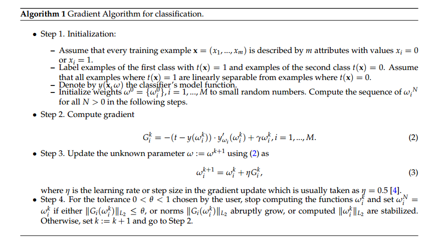
The Fréchet derivative of the functional (1) is obtained by taking \(\gamma=0\) in (7). To find optimal vector of weights \(\omega = \{\omega_i\}, i=1,...,M\) can be used the Algorithm 1 as well as least squares or machine learning algorithms.
For computation of the learning rate \(\eta\) in the Algorithm 1 usually is used optimal rule which can be derived similarly as in [14]. However, as a rule take \(\eta=0.5\) in machine learning classification algorithms [4]. Among all other regularization methods applied in machine learning [5,6,7,8,9,10,11], the regularization parameter \(\gamma\) can be also computed using the Tikhonov's theory for inverse and ill-posed problems by different algorithms presented in [15,16,17,18,19]. Some of these algorithms are discussed in Section 5.
3. Least squares for classification
The linear regression is similar to the solution of linear least squares problem and can be used for classification problems appearing in machine learning algorithms. We will revise solution of linear least squares problem in terms of linear regression.
The simplest linear model for regression is
Here, \(\omega = \{ \omega_i \}, i=0,..., M\) are weights with bias parameter \(\omega_0\), \(\{x_i\}, i=1,..., M\) are training examples. Target values (known data) are \(\{t_i\}, i=1,...,N\) which correspond to \(\{x_i\}, i=1,...,M\). Here, \(M\) is the number of weights and \(N\) is the number of data points. The goal is to predict the value of \(t\) in (1) for a new value of \(x\) in the model function (8).
The linear model (8) can be written in the form
3.1. Non-regularized least squares problem
In non-regularized linear regression or least squares problem the goal is to minimize the sum of squares
To find minimum of the error function (10) and derive the normal equations, we look for the \(\omega\) where the gradient of the norm \(\| r(\omega)\|_2^2 = ||A \omega - t||^2_2 = (A\omega - t)^T(A\omega - t)\) vanishes, or where \((\|r(\omega) \|_2^2)'_\omega =0\). To derive the Fréchet derivative, we consider the difference \(\| r(\omega + e)\|_2^2 - \| r(\omega)\|_2^2\) and single out the linear part with respect to \(\omega\). More precisely, we get
\begin{equation*} \begin{split} 0 = &{\displaystyle\lim_{\|e\| \rightarrow 0}}\dfrac{(A(\omega+e)- t)^T(A(\omega + e) - t)-(A\omega- t)^T(A\omega - t)}{||e||_2} \\ = &{\displaystyle\lim_{\|e\| \rightarrow 0}} \dfrac{((A \omega - t) + Ae )^T((A \omega - t) + Ae)-(A\omega- t)^T(A\omega - t)}{||e||_2} \\ =& {\displaystyle\lim_{\|e\| \rightarrow 0}} \dfrac{\|(A \omega - t) + Ae \|_2^2 - \| A\omega - t \|_2^2}{||e||_2} \\ &= {\displaystyle\lim_{\|e\| \rightarrow 0}} \dfrac{\|A \omega - t\|_2^2 + 2 (A \omega - t ) \cdot Ae + \| Ae \|_2^2 - \| A\omega - t \|_2^2}{||e||_2} \\ = & {\displaystyle\lim_{\|e\| \rightarrow 0}}\dfrac{2e^T(A^TA \omega - A^T t)+e^TA^TAe}{||e||_2} \end{split} \end{equation*} Thus,Equations (17) is a symmetric linear system of the \(M \times M \) linear equations for \(M\) unknowns called normal equations.
Using definition of the residual in the functionalLemma 1. The matrix \(A^T A\) is positive definite if and only if the columns of \(A\) are linearly independent, or when \(rank(A)=M\) (full rank).
Proof. We have that \(dim(A) = N \times M\), and thus, \(dim(A^T A) = M \times M\). Thus, \(\forall v \in R^M\) such that \(v \neq 0\)
For positive definite matrix \(A^TA\) we need to show that \(v^T A^T A v > 0\). Assume that \(v^T A^T A v = 0\). We observe that \(A v = 0\) only if the linear combination \(\sum_{i=1}^M a_{ji} v_i = 0\). Here, \(a_{ji}\) are elements of row \(j\) in \(A\). This will be true only if columns of \(A\) are linearly dependent or when \(v=0\), but this is contradiction with assumption \(v^T A^T A v = 0\) since \(v \neq 0\) and thus, the columns of \(A\) are linearly independent and \(v^T A^T A v > 0\).
The final conclusion is that if the matrix \(A\) has a full rank (\(rank(A)=M\)) then the system (17) is of the size \(M\)-by-\(M\) and is symmetric positive definite system of normal equations. It has the same solution \(\omega\) as the least squares problem \( \min_\omega \|A \omega - t\|^2_2\) and can be solved efficiently via Cholesky decomposition [20].
3.2. Regularized linear regression
Let now the matrix \(A\) will have entries \(a_{ij} = \phi_j(x_i), i=1,...,N; j = 1,...,M\). Recall, that functions \(\phi_j(x), j = 0,...,M\) are called basis functions which should be chosen and are known. Then the regularized least squares problem takes the form
To minimize the regularized squared residuals (20) we will again derive the normal equations. Similarly as was derived the Fréchet derivative for the non-regularized regression problem (14), we look for the \(\omega\) where the gradient of \(\frac{1}{2} ||A \omega - t||^2_2 + \frac{\gamma}{2} \| \omega \|_2^2 = \frac{1}{2} (A\omega - t)^T(A\omega - t) + \frac{\gamma}{2} \omega^T \omega\) vanishes. In other words, we consider the difference \( (\| r(\omega + e)\|_2^2 + \frac{\gamma}{2} \| \omega + e \|_2^2) - (\| r(\omega)\|_2^2 + \frac{\gamma}{2} \| \omega \|_2^2)\), then single out the linear part with respect to \(\omega\) to obtain:
\begin{equation*} \begin{split} 0 = &\frac{1}{2} {\displaystyle\lim_{\|e\| \rightarrow 0}} \dfrac{(A(\omega+e)- t)^T(A(\omega + e) - t)-(A\omega- t)^T(A\omega - t)}{||e||_2} + {\displaystyle \lim_{\|e\| \rightarrow 0}} \dfrac{\frac{\gamma}{2} (\omega +e)^T(\omega + e) - \frac{\gamma}{2} \omega^T \omega}{||e||_2} \\ =& \frac{1}{2} {\displaystyle\lim_{\|e\| \rightarrow 0}} \dfrac{\|(A \omega - t) + Ae \|_2^2 - \| A\omega - t \|_2^2}{||e||_2} + {\displaystyle\lim_{\|e\| \rightarrow 0}} \dfrac{ \frac{\gamma}{2}(\| \omega + e\|_2^2 - \| \omega \|_2^2)}{ \|e\|_2} \\ =& \frac{1}{2} {\displaystyle\lim_{\|e\| \rightarrow 0}} \dfrac{\|A \omega - t\|_2^2 + 2 (A \omega - t ) \cdot Ae + \| Ae \|_2^2 - \| A\omega - t \|_2^2}{||e||_2} + \frac{\gamma}{2} {\displaystyle\lim_{\|e\| \rightarrow 0}} \dfrac{\|\omega \|_2^2 + 2 e^T \omega + \|e \|_2^2 - \| \omega \|_2^2}{||e||_2} \end{split} \end{equation*} \begin{equation*} = \frac{1}{2} {\displaystyle\lim_{\|e\| \rightarrow 0}}\dfrac{2e^T(A^TA \omega - A^T t)+e^TA^TAe}{||e||_2} + \frac{\gamma}{2} {\displaystyle\lim_{\|e\| \rightarrow 0}}\dfrac{2e^T \omega + e^T e}{||e||_2}. \end{equation*} The termThe expression above means that the factor \(A^TA \omega - A^T t + \gamma \omega \) must also be zero, or \( (A^T A + \gamma I) \omega = A^T t, \) where \(I\) is the identity matrix. This is a system of \(M\) linear equations for \(M\) unknowns, the normal equations for regularized least squares.
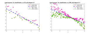
Figure 1. Least squares for classification.
3.3. Polynomial fitting to data in two-class model
Let us consider the least squares classification in the two-class model in the general case. Let the first class consisting of \(l\) points with coordinates \((x_i, y_i), i=1,...,l\) is described by it's linear modelFor creating of elements of \(A\) different basis functions can be chosen. The polynomial test functions
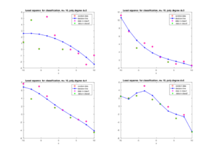
Figures 2 present examples of polynomial fitting to data for two-class model with \(m=10\) using basis functions \(\phi_j(x) =x^{j-1}, j=1,...,d\), where \(d\) is degree of the polynomial. Using these figures we observe that least squares fit data well and even can separate points in two different classes, although this is not always the case. Higher degree of polynomial separates two classes better. However, since Vandermonde's matrix can be ill-conditioned for high degrees of polynomial, we should carefully choose appropriate polynomial to fit data.
Figure 2. Least squares in polynomial fitting to data for different polynomials defined by (31).
4. Machine learning linear and polynomial classifiers
In this section we will present the basic machine learning algorithms for classification problems: perceptron learning and WINNOW algorithms. Let us start with considering of an example: determine the decision line for points presented in Figure 3. One example on this figure is labeled as positive class, another one as negative. In this case, two classes are separated by the linear equation with three weights \(\omega_i, i=1,2,3\), given by
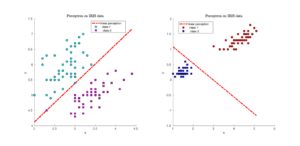
Figure 4. Decision lines computed by the perceptron learning algorithm for separation of two classes using Iris dataset [<a href=”#12″>12</a>].
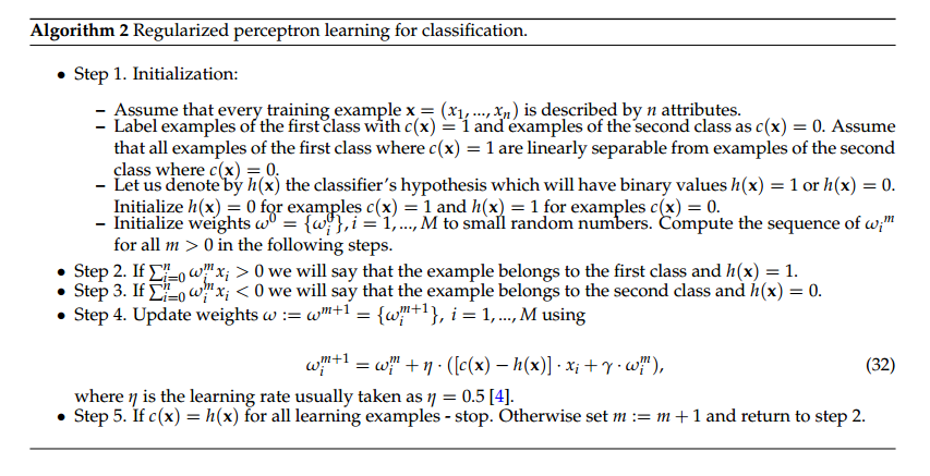
4.1. Perceptron learning for classification
The main idea of perceptron is binary classification. The perceptron computes a sum of weighted inputsBinary classifier \(y(x,\omega)\) in (37) decides whether or not an input \(x\) belongs to some specific class:
The algorithm which determines weights in (36) via binary classification (37) can be reasoned by minimization of the regularized residual
To find optimal weights in (42) we need to solve the minimization problem in the form (5)
4.2. Polynomial of the second order
Coefficients of polynomials of the second order can be obtained by the same technique as coefficients for linear classifiers. The second order polynomial function is:
Suppose that weights \(\omega_0, ..., \omega_5\) in (47) are computed. To present the decision line one need to solve the following quadratic equation for \(x_2\):
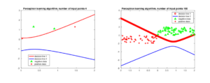
Figure 4. Perceptron learning algorithm for separation of two classes by polynomials of the second order.
4.3. WINNOW learning algorithm
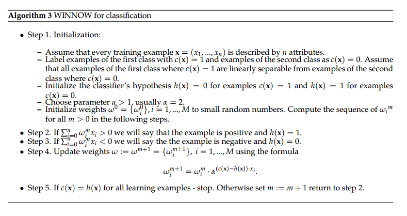
To be able compare perceptron with other machine learning algorithms, we present here one more learning algorithm which is very close to the perceptron and called WINNOW. Here is described the simplest version of this algorithm without regularization. The regularized version of WINNOW is analyzed in [22]. Perceptron learning algorithm uses additive rule in the updating weights, while WINNOW algorithm uses multiplicative rule: weights are multiplied in this rule. The WINNOW algorithm Algorithm 3 is written for \(c=t\) and \(y=h\) in (45). We will again assume that all examples where \(c(\textbf{x})=1\) are linearly separable from examples where \(c(\textbf{x})=0\).
5. Methods of Tikhonov's regularization for classification problems
To solve the regularized classification problem the regularization parameter \(\gamma\) can be chosen by the same methods which are used for the solution of ill-posed problems. For different Tikhonov's regularization strategies we refer to [15,16,17,18,19,23]. In this section we will present main methods of Tikhonov's regularization which follows ideas of [15,16,17,19,23].
Definition 2. Let \(B_{1}\) and \(B_{2}\) be two Banach spaces and \(G\subset B_{1}\) be a set. Let \(y:G\rightarrow B_{2}\) be one-to-one. Consider the equation
One can use different regularization procedures for the same classification problem. The regularization parameter \(\gamma\) can be even the vector of regularization parameters depending on number of iterations in the used classification method, the tolerance chosen by the user, number of classes, etc..
For two Banach spaces \(B_{1}\) and \(B_{2}\) let \(Q\) be another space, \(Q\subset B_{1}\) as a set and \(\overline{Q}=B_{1}\). In addition, we assume that \(Q\) is compactly embedded in \(B_{1}.\) Let \(G\subset B_{1}\) be the closure of an open set\(.\) Consider a continuous one-to-one function \(y:G\rightarrow B_{2}.\) Our goal is to solve
The regularization term \(\frac{\gamma}{2} \psi(\omega) \) encodes a priori available information about the unknown solution such that sparsity, smoothness, monotonicity, etc... Regularization term \( \frac{\gamma}{2} \psi(\omega) \) can be chosen in different norms, for example:
- \( \frac{\gamma}{2} \psi(\omega) = \frac{\gamma}{2} \| \omega \|^p_{L^p}, ~~ 1 \leq p \leq 2\).
- \(\frac{\gamma}{2} \psi(\omega) = \frac{\gamma}{2} \| \omega \|_{TV}\), TV means ``total variation''.
- \( \frac{\gamma}{2} \psi(\omega) = \frac{\gamma }{2} \| \omega \|_{BV}\), BV means ``bounded variation'', a real-valued function whose TV is bounded (finite).
- \( \frac{\gamma}{2} \psi(\omega) = \frac{\gamma }{2} \|\omega\|_{H^1}^2\).
- \( \frac{\gamma}{2} \psi(\omega) = \frac{\gamma }{2}( \|\omega \|_{L^1} + \| \omega \|^2_{L^2})\).
In this section we will discuss following rules for choosing regularization parameter in (56):
- A-priori rule (Tikhonov's regularization)
- - For \(\| t - t^*\| \leq \delta\) a priori rule requires (see details in [15]): \begin{equation*} \lim_{\delta \rightarrow 0} \gamma(\delta) \to 0, ~ \lim_{\delta \rightarrow 0} \frac{\delta^2}{\gamma(\delta)} \to 0. \end{equation*}
- A-posteriori rules:
A-priori rule and Morozov's discrepancy are most popular methods for the case when there exists estimate of the noise level \(\delta\) in data \(t\). Otherwise it is recommended to use balancing principle or other a-posteriori rules presented in [15,16,17,18,19,23].
5.1. The Tikhonov's regularization
The goal of regularization is to construct sequences \(\left\{ \gamma\left( \delta _{k}\right) \right\} ,\left\{ \omega_{\gamma \left( \delta _{k}\right) }\right\} \) in a stable way so that \begin{equation*} \lim_{k\rightarrow \infty }\left\Vert \omega_{\gamma \left( \delta _{k}\right) }- \omega^{\ast }\right\Vert _{B_{1}}=0, \end{equation*} where a sequence \(\left\{ \delta _{k}\right\} _{k=1}^{\infty }\) is such thatTo ensure (66) one can choose, for example
In [15,20] was proposed following iterative update of the regularization parameters \({\gamma_k}\) which satisfy conditions (66):
5.2. Morozov's discrepancy principle
The principle determines the regularization parameter \(\gamma=\gamma(\delta)\) in (56) such thatFor the Tikhonov functional
5.3. Balancing principle
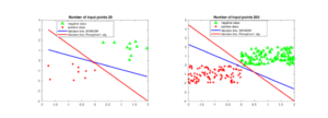
The balancing principle (or Lepskii, see [26,27]) finds \(\gamma > 0\) such that following expression is fulfilledFigure 5. Perceptron learning (red line) and WINNOW (blue line) algorithms for separation of two classes.
6. Numerical results
In this section are presented several examples which show performance and effectiveness of least squares, perceptron and WINNOW algorithms for classification. We note that all classification algorithms considered here doesn't include regularization.
6.1. Test 1
In this test the goal is to compute decision boundaries for two linearly separated classes using least squares classification. Points in these classes are generated randomly by the linear function \(y = 1.2 - 0.5x\) on different input intervals for \(x\). Then the random noise \(\delta\) is added to the data \(y(x)\) as
6.2. Test 2
Here we present examples of performance of the perceptron learning algorithm for classification of two linearly separated classes. Data for analysis in these examples are generated similarly as in the Test 1. Figures 3 present classification of two classes in the perceptron algorithm with three weights. Figures 4 show classification of two classes using the second order polynomial function 46 in the perceptron algorithm with six weights. We note that the red and blue lines presented in Figures 4 are classification boundaries computed via (51). Figures 5 present comparison of linear perceptron and WINNOW algorithms for separation of two classes. Again, all these figures show that perceptron and WINNOW algorithms can be successfully used for separation of linearly separated classes.
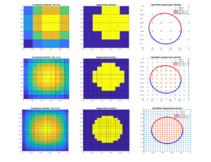
Figure 6. Classification of the computed solution for Poisson’s equation (see example 8.1.3 of [<a href=”#20″>20</a>]) on different meshes using perceptron learning algorithm.
6.3. Test 3
This test shows performance of using the second order polynomial function (46) in the perceptron algorithm for classification of the segmented solution. The classification problem in this example is formulated as follows:- Given the computed solution of the Poisson's equation
\(\triangle u = f\) with homogeneous boundary conditions \(u=0\) on the
unit square, classify the discrete solution \(u_h\) into two classes
such that the target function for classification is defined as (see middle figures of Figure 6:
\begin{equation} \label{test3_1} t_i = \left \{ \begin{array}{lll} 1, & \textrm{\({u_h}_i > 4\)} & \textrm{(yellow points)}, \\ 0, & \textrm{otherwise} & \textrm{(blue points)}. \\ \end{array} \right. \end{equation}(79)
- Use the second order polynomial function (46) in the perceptron algorithm to compute decision boundaries.
Details about setup and numerical method to compute solution of Poisson's equation are presented in the example 8.1.3 of [20]. Figure 6 presents classification of the computed solution for Poisson's equation on different meshes using second order polynomial in classification algorithm. The computed solution \(u_h\) of the Poisson's equation on different meshes is presented on the left figures of Figure 6. The middle figures show segmentation of the obtained solution satisfying (79). The right figures of Figure 6 show results of applying the second order polynomial function (46) in the perceptron algorithm for classification of the computed solution \(u_h\) with target function (79). We observe that in this particular example computed decision lines correctly separate two classes even if these classes are not linearly separable.
6.4. Test 4
In this test we show performance of linear least squares together with linear and quadratic perceptron algorithms for classification of experimental data sets: database of grey seals [13] and Iris data set [12]. Matlab code to run these simulations is available for download from the link provided in [13].
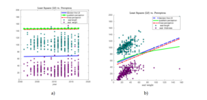
Figure 7-a) shows classification of seal length and seal weight depending on the year. Figure 7-b) shows classification of seal length and seal thickness depending on the seal weight. We observe that classes on Figure 7-a) are not linearly separable and the best algorithm which separates both classes well, is the least squares. In this example, the linear and quadratic perceptron have not classified data correctly and actually, these algorithms have not converged and stopped when the maximal number of iterations (\(10^8\)) was reached. As soon as classes become linearly separated, all algorithms show good performance and computes almost the same separation lines, see Figure 7-b).
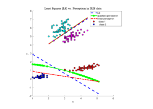
The same conclusion is obtained from separation of Iris data set [12]. Figures 8 show decision lines computed by least squares, linear and quadratic perceptron algorithms. Since all classes of Iris data set are linearly separable, all classification algorithms separate data correctly.
Figure 7. Least squares (LS) and Perceptron learning algorithm for separation of two classes using Grey Seal database [<a href=”#13″>13</a>].
Figure 9. Least squares (LS) and Perceptron learning algorithm in classification of Iris dataset [<a href=”#12″>12</a>].
7. Conclusion
We have presented regularized and non-regularized perceptron learning and least squares algorithms for classification problems as well as discussed main a-priori and a-posteriori Tikhonov's regularization rules for choosing the regularization parameter. The Fréchet derivatives for least squares and perceptron algorithms are also rigorously derived.
The future work can be related to computation of miss-classification rates which can be done similarly with works [2,29], as well as to study of classification problem using regularized linear regression, perceptron learning and WINNOW algorithms. Other classification algorithms such that regularized SVM and kernel methods can be also analyzed. Testing of all algorithms on different benchmarks as well as extension to multiclass case should be also investigated.
acknowledgments
The research is supported by the Swedish Research Council grant VR 2018-03661.conflictofinterests
The author declares no conflict of interest.References
- Bishop, C. M. (2006). Pattern recognition and machine learning. Springer.[Google Scholor]
- Hand, D. J., Mannila, H., & Smyth, P. (2001). Principles of data mining (adaptive computation and machine learning). MIT Press.[Google Scholor]
- Kotsiantis, S. B., Zaharakis, I., & Pintelas, P. (2007). Supervised machine learning: A review of classification techniques. Emerging Artificial Intelligence Applications in Computer Engineering, 160(1), 3-24.[Google Scholor]
- Kubat, M. (2017). An introduction to machine learning. Springer International Publishing AG.[Google Scholor]
- Goodfellow, I., Bengio, Y., & Courville, A. (2016). Deep learning. MIT press.[Google Scholor]
- Tsai, J. T., Chou, J. H., & Liu, T. K. (2006). Tuning the structure and parameters of a neural network by using hybrid Taguchi-genetic algorithm. IEEE Transactions on Neural Networks, 17(1), 69-80.[Google Scholor]
- Lin, S. W., Ying, K. C., Chen, S. C., & Lee, Z. J. (2008). Particle swarm optimization for parameter determination and feature selection of support vector machines. Expert Systems with Applications, 35(4), 1817-1824.[Google Scholor]
- Meissner, M., Schmuker, M., & Schneider, G. (2006). Optimized Particle Swarm Optimization (OPSO) and its application to artificial neural network training. BMC Bioinformatics, 7(1), 125.[Google Scholor]
- Bartz-Beielstein, T., Chiarandini, M., Paquete, L., & Preuss, M. (Eds.). (2010). Experimental methods for the analysis of optimization algorithms (pp. 311-336). Berlin: Springer.[Google Scholor]
- Bergstra, J., Yamins, D., & Cox, D. D. (2013, June). Hyperopt: A python library for optimizing the hyperparameters of machine learning algorithms. In Proceedings of the 12th Python in science conference (Vol. 13, p. 20). Citeseer.[Google Scholor]
- Snoek, J., Larochelle, H., & Adams, R. P. (2012). Practical bayesian optimization of machine learning algorithms. In Advances in neural information processing systems (pp. 2951-2959).[Google Scholor]
- Iris flower data set. Retrieved from {\url{https://en.wikipedia.org/wiki/Iris_flower_data_set}}[Google Scholor]
- Classification of grey seals: Matlab code and database. Retrieved from {\url{http://www.waves24.com/download}}[Google Scholor]
- Persson, C. (2016). Iteratively regularized finite element method for conductivity reconstruction in a waveguide (Master's thesis). Chalmers University of Technology.[Google Scholor]
- Bakushinsky, A. B., & Kokurin, M. Y. (2005). Iterative methods for approximate solution of inverse problems (Vol. 577). Springer Science & Business Media.[Google Scholor]
- Beilina, L., & Klibanov, M. V. (2012). Approximate global convergence and adaptivity for coefficient inverse problems. Springer Science & Business Media.[Google Scholor]
- Ito, K., & Jin, B. (2015). Inverse problems: Tikhonov theory and algorithms. Series on Applied Mathematics, World Scientific.[Google Scholor]
- Kaltenbacher, B., Neubauer, A., & Scherzer, O. (2008). Iterative regularization methods for nonlinear ill-posed problems (Vol. 6). Walter de Gruyter.[Google Scholor]
- Tikhonov, A. N., Goncharsky, A. V., Stepanov, V. V., & Yagola, A. G. (2013). Numerical methods for the solution of ill-posed problems (Vol. 328). Springer Science & Business Media.[Google Scholor]
- Beilina, L., Karchevskii, E., & Karchevskii, M. (2017). Numerical linear algebra: Theory and applications.Springer.[Google Scholor]
- Beilina, L., Thành, N. T., Klibanov, M. V., & Malmberg, J. B. (2014). Reconstruction of shapes and refractive indices from backscattering experimental data using the adaptivity. Inverse Problems, 30(10), 105007.[Google Scholor]
- Zhang, T. (2001). Regularized winnow methods. In Advances in Neural Information Processing Systems (pp. 703-709).[Google Scholor]
- Tikhonov, A. N., & Arsenin, V. Y. (1977). Solutions of ill-posed problems. New York, 1-30.[Google Scholor]
- Klibanov, M. V., Bakushinsky, A. B., & Beilina, L. (2011). Why a minimizer of the Tikhonov functional is closer to the exact solution than the first guess. Journal of Inverse and Ill-Posed Problems, 19(1), 83-105.[Google Scholor]
- Morozov, V. A. (1966). On the solution of functional equations by the method of regularization. In Doklady Akademii Nauk (Vol. 167, No. 3, pp. 510-512). Russian Academy of Sciences.[Google Scholor]
- Lazarov, R. D., Lu, S., & Pereverzev, S. V. (2007). On the balancing principle for some problems of numerical analysis. Numerische Mathematik, 106(4), 659-689.[Google Scholor]
- Mathé, P. (2006). The Lepskii principle revisited. Inverse problems, 22(3), L11-L15.[Google Scholor]
- Johnston, P. R., & Gulrajani, R. M. (1997). A new method for regularization parameter determination in the inverse problem of electrocardiography. IEEE Transactions on Biomedical Engineering, 44(1), 19-39.[Google Scholor]
- Thomas, P. (2015, November). Perceptron learning for classification problems: Impact of cost-sensitivity and outliers robustness. In 2015 7th International Joint Conference on Computational Intelligence (IJCCI) (Vol. 3, pp. 106-113). IEEE. [Google Scholor]

