Open Journal of Mathematical Sciences
ISSN: 2523-0212 (Online) 2616-4906 (Print)
DOI: 10.30538/oms2021.0159
Study of a unit power-logarithmic distribution
Christophe Chesneau
Université de Caen Normandie, LMNO, Campus II, Science 3, 14032, Caen, France; christophe.chesneau@unicaen.fr
Abstract
Keywords:
1. Introduction
Dealing with the complexities of bounded variables measuring certain characteristics of phenomenon is common in many areas of applied science. In particular, in psychology, economics, and biology, variables like proportions of a particular attribute, scores on various aptitude tests, multiple indices, and rates set on the interval \( (0, 1) \) are often encountered. Continuous probability distributions with support of \((0, 1)\), known as unit distributions, are required for an adequat modeling of these variables. The most widely used two-parameter unit distribution is the beta distribution (see [1]). When fitting data with a physical maximum, the beta distribution works great, but has some limitations in the other cases. The recent rise in the number of research papers devoted to the development of new unit interval distributions demonstrates their growing importance. Table 1 provides a quick overview of other unit distributions that have been proposed as alternatives to the beta distribution.
These distributions are dependent on one or more parameters. Their key functions have specific characteristics that are desirable in some statistical modeling context dealing with data over the interval \((0, 1)\). The majority of the recent distributions in Table 1 are created using a suitable variable transformation of a positive support baseline distribution. The main popular transformations are ratio-polynomial or exponential functions, such as \(l(x)=x/(1+x)\), \(l(x)=1/(1+x)\), or \(l(x)=e^{-x}\). Some other unit distributions are based on original analytical definitions, such as the Power (Po) distribution defined with the following cumulative distribution function (cdf):
Table 1. Some referenced unit distributions.
| Common name | Reference |
|---|---|
| Johnson \({S_B}\) | [2] |
| Topp-Leone | [3] |
| unit gamma | [4] |
| Kumaraswamy | [5] |
| standard two-sided power | [6] |
| log-Lindley | [7] |
| unit Weibull | [8, 9] |
| unit Birnbaum-Saunders | [10] |
| unit Gompertz | [11] |
| log-xgamma | [12] |
| unit inverse Gaussian | [13] |
| logit slash | [14] |
| unit generalized half normal | [15] |
| \(2^{nd}\) degree unit Lindley | [16] |
| unit Johnson SU | [17] |
| log-weighted exponential | [18] |
| unit Rayleigh | [19] |
| unit modified Burr-III | [20] |
| arcsecant hyperbolic normal | [21] |
| unit Burr-XII | [22] |
| unit power-logarithmic | [23] |
| transmuted unit Rayleigh | [24] |
| trapezoidal beta | [25] |
| unit half-normal distribution | [26] |
For the case of \(\alpha>0\), the UPL distribution was introduced and studied in-depth in [23]. For \(\alpha>0\), the properties of this distribution are as follows: (a) its pdf is defined as an original power-logarithmic scheme which is inspired by the famous Box-Cox transformation, (b) this function is increasing and can be highly asymmetric on the left, with various types of angular and J forms, which is a relatively uncommon property for a one-parameter unit distribution, (c) it has solid results in stochastic orders showing some relationship with the Po distribution, (d) its hazard rate function (hrf) is increasing, (e) simple expressions exist for a variety of moments-related quantities, such as ordinary moments, moment generating function, incomplete moments, logarithmic and logarithmically weighted moments, (f) the behavior of the moments skewness and kurtosis of the distribution is very manageable, and (g) it has a wide range of applications and can be used to build new statistical models as a generator. Despite these originalities, the main drawback of the UPL distribution is that the cdf is only defined with special integral functions; it has not a simple analytical expression. In particular, it is an obstacle for the in-depth quantile analysis of the distribution.
In this article, we contribute to the development of the power-logarithmic scheme to develop a new one-parameter unit distribution with interesting features. More precisely, we apply the power-logarithmic scheme to construct a valid cdf, instead of a power-logarithmic pdf as in the UPL distribution. As a result, the proposed distribution stands from the others by satisfying the following combined properties: (a) it is based on a single positive parameter, (b) its cdf presents various convex and concave shapes, (b) its pdf can be decreasing or U shaped, which is a relatively uncommon property for a unit distribution, (c) it has proven to be effective in stochastic orders, showing some relationship with the Po distribution, (d) it has a manageable quantile function (qf) based on the well-known Lambert function (principal branch), (e) its hrf has various types of U shapes, (f) simple expressions exist for a variety of moments-related quantities, such as ordinary moments, moment generating function, and incomplete moments, (g) the behavior of the moments skewness and kurtosis of the distribution is understable, and (h) it can perform better than the UPL and Po distributions in the context of data fitting. All these aspects are developed through mathematical, numerical and graphical investigations. We thus put the basics on a new one-parameter unit distribution that could serve in the future for various statistical objectives. As complementary results, we use the new distribution to determine some integrals linked to the Euler constant, which seem to not have received attention in the literature.
The following is the plan of the rest of the article. The new unit distribution is defined in Section 2, with analytical and graphical studies of its key functions. Section 3 is dedicated to some properties, such as diverse first order stochastic dominance, quantile analysis, and distributional results. A moment analysis is performed in Section 4. Section 5 provides some statistical perspectives of the new distribution. Complementary integral result are given in Section 6. Section 7 brings the article to a close.
2. The new power-logarithmic distribution
2.1. Presentation
The power and logarithmic functions are the main components of the proposed distribution. The following result is the key for its mathematical definition.Proposition 1. Let \(\alpha>0\). Then, the following ratio function has the properties of a continuous cdf: \begin{align*} F_{\alpha}(x)=\begin{cases}\displaystyle \frac{x^{\alpha}-1}{\alpha\log(x)} &\text{for}\ \ x\in (0,1),\\ 0 &\text{for}\ \ x\le 0,\\ 1& \text{for}\ \ x\ge 1.\end{cases} \end{align*}
Proof. By using standard asymptotic arguments, we have
\begin{align*}F_{\alpha}(x)&\underset{x\rightarrow 0}{\sim}-\frac{1}{\alpha \log(x)}\rightarrow 0,\\ F_{\alpha}(x)&=\frac{e^{\alpha \log(x)}-1}{\alpha\log(x)}\underset{x\rightarrow 1}{\sim} \frac{\alpha \log(x)}{\alpha \log(x)}=1.\end{align*} The function \(F_{\alpha}(x)\) is continuous for any \(x\in\mathbb{R}\). For any \(x\in (0,1)\), we have \begin{align*} F^{\prime}_{\alpha}(x)=\frac{\alpha x^{\alpha}\log(x)+1-x^{\alpha}}{\alpha x (\log(x))^2}. \end{align*} Owing to the following logarithmic inequality: \(\log(1+y)> y/(1+y)\), with \(y\in (-1,0)\), since \(y=x^{\alpha}-1 \in (-1,0)\) for \(x\in (0,1)\), we obtain \(\alpha \log(x)=\log(x^{\alpha})>1-1/x^{\alpha}\) which entails that \(\alpha x^{\alpha}\log(x)+1-x^{\alpha}> 0\) for \(x\in (0,1)\). Since the denominator is obviously positive too, we have \(F^{\prime}_{\alpha}(x)>0\) for any \(x\in (0,1)\), implying that \(F_{\alpha}(x)\) is strictly increasing on this interval. Therefore, \(F_{\alpha}(x)\) is increasing for \(x\in\mathbb{R}\). The proof of Proposition 1 is now complete.Thus, the cdf described in Proposition 1 defines a unit distribution, that we call the ratio power-logarithmic (RPL) distribution. When the parameter needs to be accurate, we refer to it as RPL\((\alpha)\) distribution. Even though it has a relationship with the UPL distribution, it is new to our knowledge in the literature. Indeed, one can remark that \(F_{\alpha} (x)\) is related to the pdf of the UPL distribution by the following equation:
The first notable properties of the cdf \(F_{\alpha}(x)\) are developed below.
Proposition 2. The cdf \(F_{\alpha}(x)\) is decreasing with respect to \(\alpha\), and, for any \(x\in (0,1)\), \(F_{\alpha}(x) \underset{\alpha\rightarrow 0}{=}1\) and \(F_{\alpha}(x) \underset{\alpha\rightarrow +\infty}{=}0\).
Proof. For \(x\in (0,1)\), we have
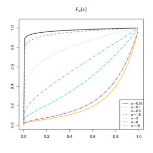
\begin{align*} \frac{\partial}{\partial \alpha}F_{\alpha}(x)=\frac{\alpha x^{\alpha}\log(x)+1-x^{\alpha}}{\alpha^2 \log(x)}=\frac{x\log(x)}{\alpha}F^{\prime}_{\alpha}(x). \end{align*} Therefore, since \(F^{\prime}_{\alpha}(x)>0\) and \(x\log(x)/\alpha< 0\), we have \(\partial F_{\alpha}(x)/\partial \alpha< 0\), and \(F_{\alpha}(x)\) is strictly decreasing with respect to \(\alpha\) for \(x\in (0,1)\), and just decreasing for \(x\in \mathbb{R}\). Furthermore, by using standard asymptotic arguments, we have \[F_{\alpha}(x)=\frac{e^{\alpha\log(x)}-1}{\alpha\log(x)}\underset{\alpha\rightarrow 0}{\sim}\frac{\alpha \log(x)}{\alpha \log(x)}=1,\] and, more directly, \[F_{\alpha}(x)\underset{\alpha\rightarrow +\infty}{\sim}-\frac{1}{\alpha\log(x)}\underset{\alpha\rightarrow +\infty}{=}0.\] The stated results are obtained.These properties are illustrated in Figure 1.
Figure 1. Plots for the cdf \(F_{\alpha}(x)\) for various values of \(\alpha\)
The various convex and concave shapes of \(F_{\alpha}(x)\) demonstrate the great modeling capacities of the RPL distribution.
2.2. Probability density function
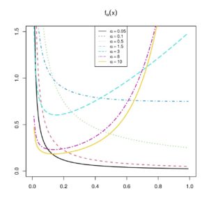
From the cdf, we easily derive the pdf of the RPL distribution as \begin{align*} f_{\alpha}(x)=F^{\prime}_{\alpha}(x)=\frac{\alpha x^{\alpha}\log(x)+1-x^{\alpha}}{\alpha x (\log(x))^2},\quad x\in (0,1), \end{align*} and \(f_{\alpha}(x) =0\) for \(x\not \in (0,1)\). Hence, for any random variable \(X\) with the RPL distribution and \(S\subseteq \mathbb{R}\), the probability that \(X\) belongs to \(S\) is given as \(\mathbb{P}(X\in S)=\int_{S} f_{\alpha}(x) dx\) and the expectation of a transformation of \(X\), say \(\ell(X)\) where \(\ell(x)\) denotes a certain function, is obtained as \(\mathbb{E}(\ell(X))=\int_{-\infty}^{+\infty}\ell(x) f_{\alpha}(x) dx\). The analytical behavior of the pdf \(f_{\alpha}(x)\) is central in the understanding of the modeling capacities of the RPL distribution. At the boundaries, the following results hold: \begin{align*} f_{\alpha}(x)&\underset{x\rightarrow 0}{\sim} \frac{1}{\alpha x (\log(x))^2} \rightarrow +\infty, \\ f_{\alpha}(x)& \underset{x\rightarrow 1}{\sim} \frac{\alpha}{2}.\end{align*} Since the derivative of \(f_{\alpha}(x)\) is complicated, we perform a graphical analysis in Figure 2 to identify the possible functional shapes.Figure 2. Plots for the pdf \(f_{\alpha}(x)\) for various values of \(\alpha\)
From Figure 2, we see that the pdf of the RPL distribution can be decreasing for the small values of \(\alpha\), or U shapes.
2.3. Other key functions
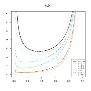
We now examine the main reliability functions of the RPL distribution. First, the survival function of the RPL distribution is obtained as \begin{align*} S_{\alpha}(x)=1-F_{\alpha}(x)=\frac{\alpha\log(x) + 1 -x^{\alpha}}{\alpha\log(x)},\quad x\in (0,1), \end{align*} \(S_{\alpha}(x) =1\) for \(x\le 0\) and \(S_{\alpha}(x) =0\) for \(x\ge 1\). From the survival function, we derive the cumulative hrf by \begin{align*} H_{\alpha}(x)& =- \log[S_{\alpha}(x)] = -\log[x^{\alpha}-1- \alpha\log(x) ] + \log(\alpha) +\log[-\log(x)] ,\quad x\in (0,1), \end{align*} and \(H_{\alpha}(x) =0\) for \(x\not \in (0,1)\). The hrf of the RPL distribution is calculated using \(H_{\alpha}(x)\) as \begin{align*} h_{\alpha}(x)=H^{\prime}_{\alpha}(x)=\frac{\alpha x^{\alpha}\log(x)+1-x^{\alpha}}{ x \log(x) [\alpha\log(x) + 1 -x^{\alpha}]},\quad x\in (0,1), \end{align*} \(h_{\alpha}(x) =0\) for \(x\not \in (0,1)\). The analytical behavior of \(h_{\alpha}(x) \) is important for understanding the statistical characteristics of the RPL distribution, especially for data fitting. We may refer to [27] and [28] for the details.Figure 3. Plots for the hrf \(h_{\alpha}(x)\) for various values of \(\alpha\)
A brief study of \(h_{\alpha}(x)\) is now provided. At the boundaries, the following results hold:
\[h_{\alpha}(x)\underset{x\rightarrow 0}{\sim} \frac{1}{\alpha x (\log(x))^2} \rightarrow +\infty, \quad h_{\alpha}(x) \underset{x\rightarrow 1}{\sim} \frac{1}{1-x}\rightarrow +\infty.\] The precise analytical behavior of \(h_{\alpha}(x)\) is difficult to analyse; its derivative is very sophisticated. As a result, we conduct a graphical analysis to comprehend its shape behavior. Figure 3 depicts some curves of \(h_{\alpha}(x)\) for various values of \(\alpha \). It is clear from Figure 3 that the hrf of the RPL distribution is exclusively U shaped.3. Some properties
Some properties satisfied by the RPL distribution are now derived.3.1. First order stochastic dominance
The first order stochastic dominance of the RPL distribution is discussed in the next proposition.Proposition 3. The following first order stochastic dominance results hold:
- 1) when \(\alpha_2\ge \alpha_1\), the RPL\((\alpha_2)\) distribution first order stochastically dominates the RPL\((\alpha_1)\) distribution,
- 2) the Po\((\alpha)\) distribution first order stochastically dominates the RPL\((\alpha)\) distribution.
Proof. Let us prove the two results in turns.
- 1) Owing to Proposition 2, \(F_{\alpha}(x)\) is decreasing with respect to \(\alpha\). Hence, for \(\alpha_2\ge \alpha_1\), we have \(F_{\alpha_2}(x)\le F_{\alpha_1}(x)\), meaning that the RPL\((\alpha_2)\) distribution first order stochastically dominates the RPL\((\alpha_1)\) distribution.
- 2) By applying the following logarithmic inequality: \(\log(1+y)< y\) for \(y> 0\), with \(y=x^{-\alpha}-1>0\) for \(x\in (0,1)\), we have \begin{align*} F_{\alpha}(x)=x^{\alpha}\frac{x^{-\alpha}-1}{\log(1+ (x^{-\alpha}-1))}> x^{\alpha}. \end{align*} Hence, for any \(x\in\mathbb{R}\), we have \(F_{\alpha}(x)\ge \mathring{F}_{\alpha}(x)\), where \(\mathring{F}_{\alpha}(x)\) is given by Equation (1), meaning that the Po\((\alpha)\) distribution first order stochastically dominates the RPL\((\alpha)\) distribution.
3.2 Quantile analysis
The quantile analysis of the RPL distribution is the focus of this section. The result below gives the expression of the qf.Proposition 4. The qf of the RPL distribution is expressed as \[Q_{\alpha}(u)=\left[-u W_{0}\left( -\frac{1}{u} e^{-1/u}\right) \right]^{1/\alpha}, \quad u\in (0,1),\] where \(W_{0}(x)\) denotes the principal branch of the Lambert function.
Proof. By its definition, the qf is \(Q_{\alpha}(u)=F^{-1}_{\alpha}(u)\) and hence satisfies the following equation: \(F_{\alpha}(y)=u\) according to \(y\). With step by step development, we obtain
\( u =F_{\alpha}(y)\ \Leftrightarrow \ u = \frac{y^{\alpha}-1}{\alpha\log(y)} \ \Leftrightarrow \ \log(y^{\alpha}) = \frac{y^{\alpha}}{u}-\frac{1}{u}\ \Leftrightarrow \ y^{\alpha}= e^{y^{\alpha}/u}e^{-1/u} \ \Leftrightarrow \ -\frac{y^{\alpha}}{u} e^{-y^{\alpha}/u}=-\frac{1}{u} e^{-1/u} \ \Leftrightarrow \ -\frac{y^{\alpha}}{u} = W_{0}\left( -\frac{1}{u} e^{-1/u}\right)\ \Leftrightarrow \ y=\left[-u W_{0}\left( -\frac{1}{u} e^{-1/u}\right) \right]^{1/\alpha}. \)The stated expression is obtained.
The next proposition is about the behavior of the qf with respect to the parameter \(\alpha\).Proposition 5. The qf \(Q_{\alpha}(u)\) is strictly increasing with respect to \(\alpha\) for \(u \in (0,1)\), and \[Q_{\alpha}(u) \underset{\alpha\rightarrow 0}{=}0, \quad Q_{\alpha}(u) \underset{\alpha\rightarrow +\infty}{=}1.\]
Proof. First, since \(Q_{\alpha}(u)\in (0,1)\) for any \(u\in (0,1)\), we have \begin{align*} \frac{\partial}{\partial \alpha}Q_{\alpha}(u)& =\frac{\partial}{\partial \alpha}e^{(1/\alpha)\log \left[-u W_{0}\left( - e^{-1/u}/u\right) \right]}\\ & =-\frac{1}{\alpha^2} \log \left[-u W_{0}\left( -\frac{1}{u} e^{-1/u}\right) \right] e^{(1/\alpha)\log \left[-u W_{0}\left( - e^{-1/u}/u\right) \right]}\\ & = -\frac{1}{\alpha} \log(Q_{\alpha}(u) ) Q_{\alpha}(u)>0. \end{align*} Therefore, \(Q_{\alpha}(u)\) is a strictly increasing function with respect to \(\alpha\) for \(u\in (0,1)\). The values of the limits are derived from the following expression: \(Q_{\alpha}(u)=v^{1/\alpha}\) with \(v=-u W_{0}\left( -e^{-1/u}/u\right) \in (0,1) \) independent of \(\alpha\); we have \(Q_{\alpha}(u) \underset{\alpha\rightarrow 0}{=}0\) and \(Q_{\alpha}(u) \underset{\alpha\rightarrow +\infty}{=}v^0=1\). Proposition 5 is proved.
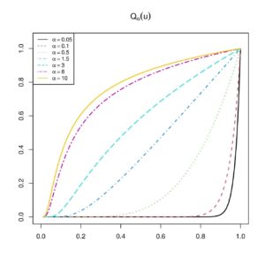
It is worth noting that the Lambert function is implemented in the majority of mathematical software, allowing the study of \(Q_{\alpha}(u)\). With the help of the library lawW of the R software (see [29]), Figure 4 depicts some curves of \(Q_{\alpha}(u)\) for several values of \(\alpha\).
Figure 4. Plots for the qf \(Q_{\alpha}(u)\) for various values of \(\alpha\)
We notice a large panel of convex and concave shapes, revealing a certain level of quantile flexibility. In addition, a clear hierarchy of the curves can be seen for increasing values of \(\alpha\), ilustrating the results in Proposition 5.
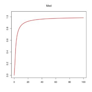
Figure 5. Plots for the median Med according to \(\alpha\)
On the other hand, Proposition 5 implies that the median defined by Med\(=Q_{\alpha}(1/2)\) is an increasing function with respect to \(\alpha\). This fact is illustrated in Figure 5.
A more in-depth quantile analysis of the RPL distribution, including the expressions of the quantile density function, hazard quantile function, quantile asymmetry and plateness measures, is possible thanks to Proposition 4. In survival studies, [30] and [31] demonstrate the importance of these quantities.
3.3. Distributional results
Let \(X\) be a random variable with the RPL\((\alpha)\) distribution. Then the following results in distribution hold.- The random variable \(Y=X^{\alpha}\) has the RPL\((1)\) distribution.
- The cdf of the random variable \(Y= b X\) with \(b>0\) is determined by \[\dot{F}_{\alpha,b}(x)=\frac{(x/b)^{\alpha}-1}{\alpha(\log(x)-\log(b))}, \quad x\in (0,b),\] \(\dot{F}_{\alpha,b}(x)=0\) for \(x\le 0\), and \(\dot{F}_{\alpha,b}(x)=1\) for \(x\ge b\). It characterizes a tuning upper bound two-parameter version of the RPL distribution.
- The cdf of the random variable \(Y= b /X\) with \(b>0\) is determined by \[\ddot{F}_{\alpha,b}(x)=1-\frac{(b/x)^{\alpha}-1}{\alpha(\log(b)-\log(x))}, \quad x>b,\] and \(\ddot{F}_{\alpha,b}(x)=0\) for \(x\le b\). It refers to a special version of the RPL distribution with a tuning lower bound.
- The cdf of the random variable \(Y=(1-X)^{1/\tau}\) with \(\tau>0\) is expressed as \[\tilde{F}_{\alpha,\tau}(x)=1-\frac{(1-x^{\tau})^{\alpha}-1}{\alpha\log(1-x^{\tau})}, \quad x\in (0,1),\] \(\tilde{F}_{\alpha,\tau}(x)=0\) for \(x\le 0\), and \(\tilde{F}_{\alpha,\tau}(x)=1\) for \(x\ge 1\). The related distribution can be considered as the RPL distribution of the second kind, proposing a new alternative unit distribution.
- The cdf of the random variable \(Y=-\log (X)\) is given as \[F^*_{\alpha}(x)=1-\frac{1-e^{-\alpha x}}{\alpha x}, \quad x>0,\] and \(F^*_{\alpha}(x)=0\) for \(x\le 0\). To our knowledge, it defines a one-parameter lifetime distribution that is not listed in the literature. It can be viewed as a new modified exponential distribution.
- The cdf of the random variable \(Y=[-\log (X)]^{1/\tau}\) with \(\tau>0\) is determined by \[F^{\circledast}_{\alpha, \tau}(x)=1-\frac{1-e^{-\alpha x^\tau}}{\alpha x^\tau}, \quad x>0,\] and \(F^{\circledast}_{\alpha, \tau}(x)=0\) for \(x\le 0\). It describes a two-parameter lifetime distribution that is not mentioned in the literature. It can be thought of as a modern version of the Weibull distribution.
- The cdf of the random variable \(Y=-\log (1-X^{\alpha})/\lambda\) with \(\lambda>0\) is specified by \[F^{\ominus}_{\lambda}(x)=-\frac{e^{-\lambda x}}{\log(1-e^{-\lambda x})}, \quad x>0,\] and \(F^{\ominus}_{\lambda}(x)=0\) for \(x\le 0\). It describes a one-parameter lifetime distribution that is not mentioned in the literature. It can be thought of as a modern version of the exponential distribution.
- The following is a generalization of the above distribution. The cdf of the random variable \(Y=\left[-\log (1-X^{\alpha})/\lambda\right]^{1/\tau}\) with \(\lambda>0\) and \(\tau>0\) is specified by \[F^{\diamond}_{\lambda,\tau}(x)=-\frac{e^{-\lambda x^\tau}}{\log(1-e^{-\lambda x^\tau})}, \quad x>0,\] and \(F^{\diamond}_{\lambda,\tau}(x)=0\) for \(x\le 0\). It describes a two-parameter lifetime distribution that has never been described before in the literature. It can be viewed a modernized version of the Weibull distribution.
- The cdf of the random variable \(Y=1/X-1\) is given as \[\breve{F}_{\alpha}(x)=1-\frac{1-(x+1)^{-\alpha}}{\alpha \log(x+1)}, \quad x>0,\] and \(\breve{F}_{\alpha}(x)=0\) for \(x\le 0\). It describes a one-parameter lifetime distribution that is not discussed in the literature. It can be thought of as a new modified Lomax distribution.
- The cdf of the random variable \(Y=\left[ (1/c)(1/X-1)\right]^{1/\tau}\) with \(\tau>0\) and \(c>0\) is obtained as \[F^{\odot}_{\alpha,\tau,c}(x)=1-\frac{1-(c x^\tau+1)^{-\alpha}}{\alpha \log(c x^\tau+1)}, \quad x>0,\] and \(F^{\odot}_{\alpha,\tau,c}(x)=0\) for \(x\le 0\). It describes a three-parameter lifetime distribution that has not been studied before. It is a new power Lomax distribution with some modifications.
- The cdf of the random variable \(Y=\sup(X_1,\ldots,X_n)\), where \(X_1,\ldots,X_n\) denote a random sample of size \(n\) derived from \(X\), is given as \begin{align*} F^{\sup}_{\alpha}(x)=\left(\frac{x^{\alpha}-1}{\alpha\log(x)}\right)^n, \quad x\in (0,1), \end{align*} \(F^{\sup}_{\alpha}(x) =0\) for \(x\le 0\) and \(F^{\sup}_{\alpha}(x) =1\) for \(x\ge 1\). In the context of order statistics theory, the related distribution is useful. From an analytical point of view, the cdf remains valid for any real number \(n>0\).
- The cdf of the random variable \(Y=\inf(X_1,\ldots,X_n)\), where \(X_1,\ldots,X_n\) denote a random sample of size \(n\) derived from \(X\), is given as \begin{align*} F^{\inf}_{\alpha}(x)=1-\left(1-\frac{x^{\alpha}-1}{\alpha\log(x)}\right)^n, \quad x\in (0,1), \end{align*} \(F^{\inf}_{\alpha}(x) =0\) for \(x\le 0\) and \(F^{\inf}_{\alpha}(x) =1\) for \(x\ge 1\). The related distribution is useful once again in the context of order statistics theory. Also, the cdf holds true for any real number \(n>0\).
- Last but not least, for a random variable \(U\) with the uniform distribution on \((0,1)\), the random variable \(Y=Q_{\alpha}(U)\) has the RPL\((\alpha)\) distribution. This result allows the generation of values from the RPL distribution based on generated values from the uniform distribution on \((0,1)\). Simulation works involving the RPL distribution are thus possible with standard methods.
4. Moments analysis
The ordinary moments of the RPL distribution are expressed in the result below.Proposition 6. Let \(X\) be a random variable with the RPL\((\alpha)\) distribution and \(r\) be a positive integer. Then, the \(r\)th ordinary moment of \(X\) is obtained as \begin{align*} m_{\alpha}(r)=\mathbb{E}(X^r)=1 - \frac{r}{\alpha}\log\left(1+\frac{\alpha}{r}\right). \end{align*} The case \(r=0\) is not covered by this formula, but we can set \(m_{\alpha}(0)=\mathbb{E}(X^0)=1\).
Proof. Through the integral definition of the \(r\)th ordinary moment, we have \[m_{\alpha}(r)=\int_{-\infty}^{+\infty}x^r f_{\alpha}(x)dx=\frac{1}{\alpha}\int_{0}^{1}x^{r-1} \frac{\alpha x^{\alpha}\log(x)+1-x^{\alpha}}{(\log(x))^2} dx.\] Let us now introduce the following function of \(\alpha\): \begin{align*} \Psi_{r}(\alpha)&=\int_{0}^{1}x^{r-1} \frac{\alpha x^{\alpha}\log(x)+1-x^{\alpha}}{(\log(x))^2} dx, \end{align*} with \(\Psi_{r}(\alpha)=0\) for \(\alpha=0\). By applying the Leibnitz integral rule, we get \begin{align*} \frac{\partial}{\partial \alpha}\Psi_{r}(\alpha)&= \frac{\partial}{\partial \alpha}\int_{0}^{1}x^{r-1} \frac{\alpha x^{\alpha}\log(x)+1-x^{\alpha}}{(\log(x))^2} dx =\int_{0}^{1}x^{r-1} \frac{1}{(\log(x))^2}\frac{\partial}{\partial \alpha} (\alpha x^{\alpha}\log(x)+1-x^{\alpha}) dx\\ & = \int_{0}^{1}x^{r-1}\frac{1}{(\log(x))^2} \times \alpha x^{\alpha } (\log(x))^2dx= \alpha \int_{0}^{1}x^{r+\alpha-1}dx=\frac{\alpha}{r+\alpha}=1- \frac{r}{r+\alpha}. \end{align*} Upon integrating with respect to \(\alpha\), we obtain \(\Psi_{r}(\alpha)=\alpha - r\log(r+\alpha)+c\), where \(c\) denotes a generic constant at this step. Since \(\Psi_{r}(0)=0\), we have \(c=r\log(r)\). Therefore \[\Psi_{r}(\alpha)=\alpha - r\log(r+\alpha)+r\log(r)=\alpha - r\log\left(1+\frac{\alpha}{r}\right).\] Hence \[m_{\alpha}(r)=\frac{1}{\alpha}\Psi_{r}(\alpha)=1 - \frac{r}{\alpha}\log\left(1+\frac{\alpha}{r}\right),\] ending the proof of Proposition 6.
Alternative approach
Another approach consists of using the alternative formula: \(m_{\alpha}(r)=r \int_{0}^{+\infty}x^{r-1} S_{\alpha}(x)dx\), and Equation (3) as follows: \begin{align*} m_{\alpha}(r)& =r \int_{0}^{+\infty}x^{r-1} S_{\alpha}(x)dx\\ &=r \int_{0}^{1}x^{r-1}dx -r \int_{0}^{1}x^{r-1} F_{\alpha}(x)dx\\ & = 1 -r\frac{\log(1+\alpha)}{\alpha} \int_{0}^{1}x^{r-1} f^{┼}_{\alpha}(x)dx\\ &= 1 -r\frac{\log(1+\alpha)}{\alpha} \mathbb{E}(Y^{r-1}), \end{align*} where \(Y\) denotes a random variable with the UPL distribution. By virtue of [23, Proposition 3.1], we have \(\mathbb{E}(Y^{r-1})=\log\left( 1+{\alpha}/{r}\right)/\log(1+\alpha)\), implying the desired result.Some properties of the ordinary moments are expressed in the next result.
Proposition 7. The following properties of the ordinary moments hold:
- 1) \(m_{\alpha}(r)\) is a strictly increasing function with respect to \(\alpha\),
- 2) \(m_{\alpha}(r)\) is a strictly decreasing function with respect to \(r\).
Proof.
- 1) Since \(\log(1+y)>y/(1+y)\) for \(y>0\), by taking \(y=\alpha/r>0\), we have \[\frac{\partial}{\partial \alpha}m_{\alpha}(r) =\frac{r}{\alpha^2 (\alpha+r)}\left[ (\alpha+r)\log\left(1+\frac{\alpha}{r}\right)-\alpha \right]>0,\] implying that \(m_{\alpha}(r)\) is a strictly increasing function with respect to \(\alpha\).
- 2) With the same justification, we have \[\frac{\partial}{\partial r} m_{\alpha}(r)= \frac{1}{\alpha (\alpha+r)}\left[\alpha- (\alpha+r)\log\left(1+\frac{\alpha}{r}\right) \right] < 0,\] entailing that \(m_{\alpha}(r)\) is a strictly decreasing function with respect to \(r\). Or, since the support of \(X\) is \((0,1)\), it is clear that \(W_r=X^r\) is a decreasing sequence of random variables, implying the decreasingness of \( m_{\alpha}(r)\).
This ends the proof of Proposition 7.
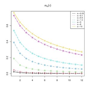
We now illustrate the findings of Proposition 7 in Figure 6, by plotting \(m_r(\alpha)\) for various values of \(r\) and \(\alpha\).
Figure 6. Plots for the moments \(m_{\alpha}(r)\) for various values of \(\alpha\) and \(r\)
From this figure, we clearly see that \(m_{\alpha}(r)\) is a strictly increasing function with respect to \(\alpha\), and a strictly decreasing function with respect to \(r\).
Based on Proposition 6, the mean of \(X\) is given as
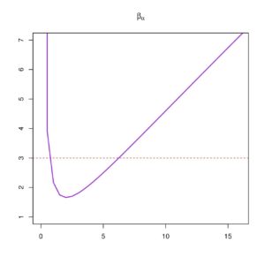
\[m_{\alpha}=m_{\alpha}(1)=\mathbb{E}(X)=1 - \frac{1}{\alpha}\log\left(1+\alpha\right)\] and the variance of \(X\) is obtained as \begin{align*} \sigma_{\alpha}^2& = \mathbb{V}(X)=m_{\alpha}(2)-m_{\alpha}(1)^2=1 - \frac{2}{\alpha}\log\left(1+\frac{\alpha}{2}\right) - m_{\alpha}^2\\ & =\frac{1}{\alpha^2}\left[ 2\alpha \log(1+\alpha)-\log(1+\alpha)^2-2\alpha \log\left(1+\frac{\alpha}{2}\right) \right]. \end{align*} Also, the skewness and kurtosis coefficients of \(X\) are given as \begin{align*} \gamma_{\alpha}=\frac{m_{\alpha}(3)-3m_{\alpha} \sigma_{\alpha}^2-m_{\alpha}^3}{\sigma_{\alpha}^3}, \quad \beta_{\alpha}=\frac{m_{\alpha}(4)-4m_{\alpha}(3) m_{\alpha}+6m_{\alpha}(2) m_{\alpha}^2-3 m_{\alpha}^4}{\sigma_{\alpha}^4}, \end{align*}respectively. In our context, \(\gamma_{\alpha}\) is a measure of relative symmetry, and \(\beta_{\alpha}\) is a measure of the relative peakedness of the RPL distribution. Figure 7 presents the curves for \(\gamma_{\alpha}\) and \(\beta_{\alpha}\) with respect to \(\alpha\).
Figure 7. Plots for (a) \(\gamma_{\alpha}\) and (b) \(\beta_{\alpha}\) with respect to \(\alpha\)
From this figure, one can remark that \(\gamma_{\alpha}\) is a strictly decreasing function with respect to \(\alpha\), and can be negative or positive, meaning that the RPL distribution can be left or right skewed, respectively. Also, we note that \(\beta_{\alpha}\) is a non-monotonic function with a ``skewed V'' shape. In addition, it can be inferior, equal or superior to \(3\), meaning that the RPL distribution may be platykurtic, mesokurtic, or leptokurtic, respectively.
We now discuss the moment generating function of the RPL distribution.
Proposition 8. Let \(X\) be a random variable with the RPL\((\alpha)\) distribution and \(t\in\mathbb{R}\). Then, the moment generating function of \(X\) is obtained as \begin{align*} M_{\alpha}(t) =e^t - \frac{t}{\alpha}\sum_{k=0}^{+\infty}\frac{t^k}{k!} \log\left(1+\frac{\alpha}{k+1}\right). \end{align*}
Proof. By using the Taylor series of the exponential function combined with Proposition 6, we get \begin{align*} M_{\alpha}(t)& =\mathbb{E}(e^{tX})=1+\sum_{k=1}^{+\infty}\frac{t^k}{k!}m_{\alpha}(k)=1+\sum_{k=1}^{+\infty}\frac{t^k}{k!} \left[ 1 - \frac{k}{\alpha}\log\left(1+\frac{\alpha}{k}\right)\right] \\ & =1+\sum_{k=1}^{+\infty}\frac{t^k}{k!} - \frac{1}{\alpha}\sum_{k=1}^{+\infty}\frac{t^k}{(k-1)!} \log\left(1+\frac{\alpha}{k}\right)=e^t - \frac{t}{\alpha}\sum_{k=0}^{+\infty}\frac{t^k}{k!} \log\left(1+\frac{\alpha}{k+1}\right). \end{align*} The desired formula is obtained.
As a consequence of Proposition 8, we have
\begin{align*} M_{\alpha}(r,t)=\mathbb{E}(X^r e^{tX})=\frac{\partial^r }{\partial t^r}M_{\alpha}(t)&= e^t - \frac{1}{\alpha}\sum_{k=r-1}^{+\infty}\frac{k+1}{(k-r+1)!} t^{k-r+1} \log\left(1+\frac{\alpha}{k+1}\right). \end{align*} This formula can be applied for any chosen value of \(t\). The following relationship can be used to obtain the \(r \)th ordinary moment: \(m_{\alpha}(r)=M_{\alpha}(r,0)\).The incomplete moments of the RPL distribution are now expressed.
Proposition 9. Let \(X\) be a random variable with the RPL\((\alpha)\) distribution, \(r\) be a positive integer, and \(X_t\) be the truncated version of \(X\) at a threshold \(t\) with \(t\in [0,1]\). Then, the \(r\)th incomplete moment of \(X\) at \(t\) is obtained as the \(r\)th ordinary moment of \(X_t\), that is \begin{align*} m_{\alpha}(r, t)=\mathbb{E}(X_t^r)= t^rF_{\alpha}(t)-\frac{r}{\alpha} \left\lbrace Ei[ (\alpha+r)\log(t)]- Ei[ r\log(t)] \right\rbrace, \end{align*} where \(Ei(x)\) is the exponential integral defined by \[Ei(x)=\int_{-\infty}^x\frac{e^{t }}{t}dt, \quad x\in \mathbb{R}^*.\]
Proof. We proceed as for the proof of Proposition 6. We have \[m_{\alpha}(r, t)=\int_{-\infty}^{t}x^r f_{\alpha}(x)dx=\frac{1}{\alpha}\int_{0}^{t}x^{r-1} \frac{\alpha x^{\alpha}\log(x)+1-x^{\alpha}}{(\log(x))^2} dx.\] Now, let us consider the following function: \begin{align*} \Psi_{r}(\alpha,t)&=\int_{0}^{t}x^{r-1} \frac{\alpha x^{\alpha}\log(x)+1-x^{\alpha}}{(\log(x))^2} dx, \end{align*} with \(\Psi_{r}(\alpha,t)=0\) for \(\alpha=0\). By applying the Leibnitz integral rule, we get \begin{align*} \frac{\partial}{\partial \alpha}\Psi_{r}(\alpha,t)&=\frac{\partial}{\partial \alpha} \int_{0}^{t}x^{r-1} \frac{\alpha x^{\alpha}\log(x)+1-x^{\alpha}}{(\log(x))^2} dx =\int_{0}^{t}x^{r-1} \frac{1}{(\log(x))^2}\frac{\partial}{\partial \alpha} (\alpha x^{\alpha}\log(x)+1-x^{\alpha}) dx\\ & = \int_{0}^{t}x^{r-1}\frac{1}{(\log(x))^2} \times \alpha x^{\alpha } (\log(x))^2dx= \alpha \int_{0}^{t}x^{r+\alpha-1}dx=\frac{\alpha}{r+\alpha}t^{r+\alpha}. \end{align*} Now, by an integration with respect to \(\alpha\) and suitable changes of variables, we obtain \begin{align*} \int_{0}^{\alpha}\frac{u}{r+u}t^{r+u} du&= t^{r}\int_{0}^{\alpha} t^{u}du-r \int_{0}^{\alpha} \frac{t^{r+u}}{r+u}du \\ & =t^r\frac{t^{\alpha}-1}{\log(t)}-r \int_{r}^{\alpha+r} \frac{t^{v}}{v}dv =t^r\frac{t^{\alpha}-1}{\log(t)}-r \int_{r\log(t)}^{(\alpha+r)\log(t)} \frac{e^{w}}{w}dw \\ & = \alpha t^rF_{\alpha}(t)-r \left\lbrace Ei[ (\alpha+r)\log(t)]- Ei[ r\log(t)] \right\rbrace. \end{align*} Therefore, \(\Psi_{r}(\alpha,t)= \alpha t^rF_{\alpha}(t)-r \left\lbrace Ei[ (\alpha+r)\log(t)]- Ei[ r\log(t)] \right\rbrace+c\), where \(c\) denotes a certain constant satisfying \(\Psi_{r}(0,t)=0\), that is, \(c=0\). Therefore \[\Psi_{r}(\alpha,t)= \alpha t^rF_{\alpha}(t)-r \left\lbrace Ei[ (\alpha+r)\log(t)]- Ei[ r\log(t)] \right\rbrace.\] Hence \[m_{\alpha}(r, t)=\frac{1}{\alpha}\Psi_{r}(\alpha,t)=t^rF_{\alpha}(t)-\frac{r}{\alpha} \left\lbrace Ei[ (\alpha+r)\log(t)]- Ei[ r\log(t)] \right\rbrace,\] ending the proof of Proposition 9.
From Proposition 9, we refind the \(r\)th ordinary moment of \(X\) by the limit technique; since
\begin{align*} t^rF_{\alpha}(t)\underset{t\rightarrow 1}{=}1, \quad Ei[ (\alpha+r)\log(t)]- Ei[ r\log(t)] \underset{t\rightarrow 1}{=}\log\left( 1+\frac{\alpha}{r}\right), \end{align*} we obtain \begin{align*} m_{\alpha}(r)\underset{t\rightarrow 1}{=}m_{\alpha}(r, t)=1 - \frac{r}{\alpha}\log\left(1+\frac{\alpha}{r}\right). \end{align*} We mention that the incomplete moments are used in a variety of essential probability functions, including the residual life function and its ordinary moments, the respected residual life function and its ordinary moments, the Lorenz, Zenga and Bonferroni curves, and so on. On this topic, we may refer to [32].5. Statistical perspective
Let us now consider the setting of the RPL\((\alpha)\) distribution, assuming that the parameter \(\alpha\) is unknown. Mathematically, the maximum likelihood estimate (MLE) of \(\alpha\) is obtained as \(\hat \alpha=argmax_{\alpha\in (0,+\infty)}L_{\alpha}\), where \[L_{\alpha}=\prod_{i=1}^n f_{\alpha}(x_i)=\prod_{i=1}^n\frac{\alpha x_i^{\alpha}\log(x_i)+1-x_i^{\alpha}}{\alpha x_i (\log(x_i))^2},\] and \(x_1,\ldots,x_n\) denote \(n\) values of a certain variable with support in \((0,1)\), representing data which are ideally the realizations of a random variable with the RPL\((\alpha)\) distribution. Therefore, for any \(\beta>0\), the MLE \(\hat \alpha\) is such that \(L_{\beta}\le L_{\hat \alpha}\). Many and well-known convergence properties underpin the random estimator of \(\hat \alpha\). We may refer to the general theory in [33] for more information on this matter.We intend to demonstrate that the RPL distribution can provide better results than the comparable one-parameter UPL and Po distributions for some types of data and with the use of MLEs. We recall that the functions in Equations (2) and (1) specified these two last distributions, respectively. For comparison, we use established statistical criteria, such as the Akaike information criterion (AIC), corrected Akaike information criterion (AICc) and Bayesian information criterion (BIC), defined by \(\text{AIC} = -2 \log L_{\hat{\alpha}} + 2 k\), \(\text{AICc}=\text{AIC}+2 k (k+1)/(n-k-1)\) and \(\text{BIC} = -2 \log L_{\hat{\alpha}}+ k \log(n)\), respectively, where \(k\) is the number of parameters to be estimated. For the considered distributions, since there is only one parameter, we take \(k=1\). The distribution with the smallest AIC, AICc, or BIC is considered to have the best fit of the data.
Here, we generate four different data sets presenting U or J shapes. More precisely, each data set contains \(200\) values which are realisations of the following random variable: \(X=1/(1+Y)\), where \(Y\) is a random variable with the Pareto distribution specified by the following pdf: \(f^{\flat}_{\upsilon, \theta}(x)=\theta \upsilon^{\theta}x^{-(\theta+1)}\), \(x\ge \upsilon\), and \(f^{\flat}_{\upsilon, \theta}(x)=0\) for \(x< \upsilon\), where \(\upsilon>0\) and \(\theta>0\). For the \(j\)th data set, called Data set \(j\), we consider the following parameters: \(\upsilon=2^{-(j+2)}\) and \(\theta=(j+2)^{-1/2}\) with \(j=1,2,3,4\).
The considered criteria for the three distributions are given in Table 2, for each data set. In all the calculations, the R software is used, and all the codes are available upon author request.
Table 2. Criteria related to the RPL, UPL and Po distributions for Data sets 1, 2, 3 and 4.
| Data set 1 | MLE \(\hat \alpha\) | AIC | AICc | BIC |
|---|---|---|---|---|
| RPL | 4.612479 | -36.65037 | -36.63017 | -33.35205 |
| UPL | 2.148819 | -26.77903 | -26.75883 | -23.48071 |
| Po | 1.374657 | -16.26337 | -16.24317 | -12.96506 |
| Data set 2 | ||||
| RPL | 6.653810 | -105.23541 | -105.21521 | -101.93710 |
| UPL | 6.294888 | -57.57819 | -57.55799 | -54.27987 |
| Po | 1.344703 | -13.93269 | -13.91249 | -10.63437 |
| Data set 3 | ||||
| RPL | 11.298643 | -225.40800 | -225.38780 | -222.10968 |
| UPL | 16.288507 | -174.03556 | -174.01536 | -170.73724 |
| Po | 1.696079 | -45.16569 | -45.14549 | -41.86737 |
| Data set 4 | ||||
| RPL | 16.280371 | -301.34203 | -301.32183 | -298.04371 |
| UPL | 34.643019 | -229.43869 | -229.41849 | -226.14037 |
| Po | 1.471506 | -24.34491 | -24.32471 | -21.04659 |
In this table, the smallest values of AIC, AICc, and BIC are obtained for the RPL distribution; it can be considered as the best.
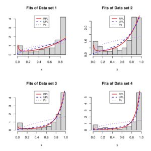
Figure 8. Examples of data fitting via the three considered distributions
In the setting of the RPL distribution, based on the MLE \(\hat \alpha\), the estimated pdf is given by \(\hat f(x)=f_{\hat \alpha}(x)\). We can define the estimated pdfs of the UPL and Po distributions in a similar manner. Figure 8 shows how these estimated pdfs fit the histogram of the data.
From this figure, we see that the RPL distribution has well captured the U or J shapes of the histograms, and especially the data to the left corresponding to \(x\in (0, 0.1)\), which is not the case of the two competitors.
6. Complement: around the Euler constant
The next result provides a new parametric integral result which can be proven by using the RPL distribution, among other techniques.Proposition 10. Let \(\alpha>0\). Then the following equality holds: \begin{align*} \int_{0}^{1}\frac{\log(1-x)}{x (\log(x))^2} \left[x^{\alpha}(1-\alpha \log(x))-1\right]dx=& \alpha \gamma + \log[\Gamma(\alpha+1)], \end{align*} where \(\gamma\) is the Euler constant and \(\Gamma(x)\) is the standard gamma function.
Proof. We will prove this result by using the moments of the RPL distribution. For any random variable \(X\) following the RPL distribution and any positive integer \(k\), it comes from Proposition 6 that \[\frac{1}{k}\mathbb{E}(X^k)=\frac{1}{k} - \frac{1}{\alpha}\log\left(1+\frac{\alpha}{k}\right).\] It follows from this relation, the Lebesgue dominated convergence theorem and the series expansion of the logarithmic function that
A new integral expression of the Euler constant comes from Proposition 10; by taking \(\alpha=1\), we get
\begin{align*} \gamma = \int_{0}^{1}\frac{\log(1-x)}{x (\log(x))^2} \left[x(1-\log(x))-1\right]dx. \end{align*} As far as we know, this integral form of the Euler constant is not listed in the literature, at least under this form. In particular, it dont appear in the indispensable book of [34]. Some relationships with existing integrals are formulated below.- The result [34, 4.283(7)] states that \begin{align*} \gamma=\int_{0}^{1}\frac{1}{x \log(x)(1-\log(x))} \left[x(1-\log(x))-1\right]dx. \end{align*} Hence we have \(\gamma=\int_{0}^{1}u(x)\left[x(1-\log(x))-1\right]/(x\log(x))dx\) with \(u(x)=1/(1-\log(x))\) and, thanks to Proposition 10, this is also valid for the function: \(u(x)=\log(1-x)/\log(x)\).
- The result [34, 4.314(3)] states that \begin{align*} \int_{0}^{1}\frac{\log(1+x)}{x (\log(x))^2} \left[x(1-\log(x))-1\right]dx=\log\left(\frac{\pi}{4}\right). \end{align*} Thus, in comparison to the integral in Proposition 10, only the term \(\log(1+x)\) has been changed to \(\log(1-x)\), with a surprising consequence. The following integral can be deduced by summation: \begin{align*} \int_{0}^{1}\frac{\log(1-x^2)}{x (\log(x))^2} \left[x(1-\log(x))-1\right]dx=\gamma+\log\left(\frac{\pi}{4}\right). \end{align*}
The next result is derived to Proposition 10, and also appears in [35].
Proposition 11. Let \(\alpha>0\). Then the following equality holds: \begin{align*} \int_{0}^{1}\frac{1}{(1-x)\log(x)}[\alpha\log(x) + 1 -x^{\alpha}]dx= \alpha \gamma + \log[\Gamma(\alpha+1)]. \end{align*}
Proof. We follow the spirit of the proof of Proposition 10, with the same notations. By using Equations (6) and (4), applying an integration by part and using \(S_{\alpha}(x)\underset{x\rightarrow 1}{\sim}\alpha(1-x)/2\), we get \begin{align*} \gamma + \frac{1}{\alpha}\log[\Gamma(\alpha+1)]&= \sum_{k=1}^{+\infty}\left[\frac{1}{k} - \frac{1}{\alpha}\log\left(1+\frac{\alpha}{k}\right) \right]=\mathbb{E}\left(-\log(1-X)\right) = \int_{0}^{1}[-\log(1-x)]f_{\alpha}(x)dx\\ & = [-\log(1-x)](-S_{\alpha}(x)) \mid_{x=0}^1+\int_{0}^{1}\frac{1}{1-x}S_{\alpha}(x)dx\\ & =0+ \int_{0}^{1}\frac{1}{1-x}\frac{\alpha\log(x) + 1 -x^{\alpha}}{\alpha\log(x)}dx, \end{align*} implying that \begin{align*} &\int_{0}^{1}\frac{1}{(1-x)\log(x)}[\alpha\log(x) + 1 -x^{\alpha}]dx= \alpha \gamma + \log[\Gamma(\alpha+1)]. \end{align*} The desired outcome is achieved.
In [35], the proof is completely different; it is based on a parametric derivative-sum-integral technique.
The above findings may be used for a variety of purposes, beyond the scope of the article.
7. Concluding remarks
7.1. Conclusion
This article has presented a new unit distribution whose cdf is constructed from a one-parameter power-logarithmic scheme. It is called the ratio power-logarithmic (RPL) distribution. We have highlighted the great flexibility of the corresponding cdf, characterized by a large selection of convex and concave shapes. The other key functions are determined and studied. In particular, we have shown that the pdf may take on different decreasing or U shapes, and the hrf has a wide panel of U shapes. These functional capabilities are rare enough to motivate the interest of the RPL distribution. Furthermore, we established certain stochastic order results, and provided the qf expression via the Lambert function, some interesting distributional results, and simple expressions for various moments. Then, in the framework of the data analysis, a simple statistical approach to the new distribution has been defined. Finally, complementary mathematical results have been demonstrated using specific moments properties of the RPL distribution, giving new integrals connected with the Euler constant.7.2. Future research prospects
Based on the current work, the future research prospects are numerous, including the development of the RPL generated family of distributions defined with the following cdf: \[F^G_{\alpha}(x)=F_{\alpha} (G (x))=\frac{(G(x))^{\alpha}-1}{\alpha\log(G(x))}, \quad x\in\mathbb{R},\] where \(G (x)\) denotes any generic cdf of a continuous distribution, the construction of regression models based on unit distributions (quantile regression, mean regression...), and multivariate extensions. Each of these topics has theoretical and practical potential to meet modern statistical needs. However, they require further development, which we have deferred for the time being.Conflicts of Interest: The author declares no conflict of interest.
Data Availability: The data required for this research are simulated data. The code is available on request from the author.
Funding Information: No funding is available for this research.
Acknowledgments: The author is thankful to the two anonymous referees for their constructive comments.
References
- Ferrari, S. L., & Cribari-Neto, F. (2004). Beta regression for modelling rates and proportions. Journal of Applied Statistics, 31(7), 799-815. [Google Scholor]
- Johnson, N. L. (1949). Systems of frequency curves generated by methods of translation. Biometrika, 36(1/2), 149-176. [Google Scholor]
- Topp, C. W., & Leone, F. C. (1955). A family of J-shaped frequency functions. Journal of the American Statistical Association, 50(269), 209-219. [Google Scholor]
- Consul, P. C., & Jain, G. C. (1971). On the log-gamma distribution and its properties. Statistical Papers, 12, 100-106. [Google Scholor]
- Kumaraswamy, P. (1980). A generalized probability density function for double-bounded random processes. Journal of Hydrology, 46(1-2), 79-88. [Google Scholor]
- Van Dorp, J. R., & Kotz, S. (2002). The standard two-sided power distribution and its properties: with applications in financial engineering. The American Statistician, 56(2), 90-99.[Google Scholor]
- Gómez-Déniz, E., Sordo, M. A., & Calderín-Ojeda, E. (2014). The log-Lindley distribution as an alternative to the beta regression model with applications in insurance. Insurance: Mathematics and Economics, 54, 49-57.[Google Scholor]
- Mazucheli, J., Menezes, A. F. B., & Ghitany, M. E. (2018). The unit-Weibull distribution and associated inference. Journal of Applied Probability and Statistics, 13, 1-22. [Google Scholor]
- Mazucheli, J., Menezes, A. F. B., Fernandes, L. B., de Oliveira, R. P., & Ghitany, M. E. (2020). The unit-Weibull distribution as an alternative to the Kumaraswamy distribution for the modeling of quantiles conditional on covariates. Journal of Applied Statistics, 47(6), 954-974. [Google Scholor]
- Mazucheli, J., Menezes, A. F., & Dey, S. (2018). The unit-Birnbaum-Saunders distribution with applications. Chilean Journal of Statistics, 9(1), 47-57. [Google Scholor]
- Mazucheli, J., Menezes, A. F., & Dey, S. (2019). Unit-Gompertz distribution with applications. Statistica, 79(1), 25-43. [Google Scholor]
- Altun, E., & Hamedani, G. G. (2018). The log-xgamma distribution with inference and application. Journal de la Société Française de Statistique, 159(3), 40-55. [Google Scholor]
- Ghitany, M. E., Mazucheli, J., Menezes, A. F. B., & Alqallaf, F. (2019). The unit-inverse Gaussian distribution: A new alternative to two-parameter distributions on the unit interval. Communications in Statistics-Theory and Methods, 48(14), 3423-3438. [Google Scholor]
- Korkmaz, M. Ç. (2020). A new heavy-tailed distribution defined on the bounded interval: the logit slash distribution and its application. Journal of Applied Statistics, 47(12), 2097-2119. [Google Scholor]
- Korkmaz, M. Ç. (2020). The unit generalized half normal distribution: A new bounded distribution with inference and application. University Politehnica of Bucharest Scientific Bulletin-Series A-Applied Mathematics and Physics, 82(2), 133-140. [Google Scholor]
- Altun, E., & Cordeiro, G. M. (2020). The unit-improved second-degree Lindley distribution: inference and regression modeling. Computational Statistics, 35(1), 259-279. [Google Scholor]
- Gündüz, S., & Korkmaz, M. Ç. (2020). A new unit distribution based on the unbounded Johnson distribution rule: The unit Johnson SU distribution. Pakistan Journal of Statistics and Operation Research, 16(3), 471-490. [Google Scholor]
- Altun, E. (2020). The log-weighted exponential regression model: alternative to the beta regression model. Communications in Statistics-Theory and Methods, https://doi.org/10.1080/03610926.2019.1664586 [Google Scholor]
- Bantan, R. A. R., Chesneau, C., Jamal, F., Elgarhy, M., Tahir, M. H., Aqib, A., Zubair, M., & Anam, S. (2020). Some new facts about the unit-Rayleigh distribution with applications. Mathematics, 8(11), Article No 1954. [Google Scholor]
- Haq, M. A., Hashmi, S., Aidi, K., Ramos, P. L., & Louzada, F. (2020). Unit modified Burr-III distribution: Estimation, characterizations and validation test. Annals of Data Science, to appear. https://doi.org/10.1007/s40745-020-00298-6 [Google Scholor]
- Korkmaz, M. Ç., Chesneau, C., & Korkmaz, Z. S. (2021). On the arcsecant hyperbolic normal distribution. Properties, quantile regression modeling and applications. Symmetry, 13(1), Article No 117. [Google Scholor]
- Korkmaz, M. Ç., & Chesneau, C. (2021). On the unit Burr-XII distribution with the quantile regression modeling and applications. Computational and Applied Mathematics, 40(29), 1-26. [Google Scholor]
- Chesneau, C. (2021). A note on an extreme left skewed unit distribution: Theory, modelling and data fitting. Open Statistics, To appear.
- Korkmaz, M. Ç., Chesneau, C., & Korkmaz, Z. S. (2021). Transmuted unit Rayleigh quantile regression model: alternative to beta and Kumaraswamy quantile regression models. University Politehnica of Bucharest Scientific Bulletin-Series A-Applied Mathematics and Physics, To appear. [Google Scholor]
- Figueroa-Zu, J. I., Niklitschek-Soto, S. A., Leiva, V., & Liu, S. (2021). Modeling heavy-tailed bounded data by the trapezoidal beta distribution with applications, Revstat, To appear. [Google Scholor]
- Bakouch, H. S., Nik, A. S., Asgharzadeh, A., & Salinas, H. S. (2021). A flexible probability model for proportion data: Unit-half-normal distribution. Communications in Statistics-Case Studies, Data Analysis and Applications, DOI:10.1080/23737484.2021.1882355 [Google Scholor]
- Aarset, M. V. (1987). How to identify bathtub hazard rate. IEEE Transactions Reliability, 36, 106-108. [Google Scholor]
- Lee, E. T. (1992). Statistical Methods for Survival Data Analysis, John Wiley, New York. [Google Scholor]
- R Core Team (2014). R: A language and environment for statistical computing. R Foundation for Statistical Computing, Vienna, Austria. URL http://www.R-project.org/. [Google Scholor]
- Gilchrist, W. (2000). Statistical Modelling with Quantile Functions. CRC Press, Abingdon. [Google Scholor]
- Nair, N. U., & Sankaran, P. G. (2009). Quantile based reliability analysis. Communications in Statistics: Theory and Methods, 38(2), 222-232. [Google Scholor]
- Butler, R. J., & McDonald, J. B. (1989). Using incomplete moments to measure inequality. Journal of Econometrics, 42, 109-119. [Google Scholor]
- Casella, G., & Berger, R. L. (1990). Statistical Inference, Brooks/Cole Publishing Company: Bel Air, CA, USA.
- Gradshteyn, I. S., & Ryzhik, I. M. (2007). Table of Integrals, Series, and Products, Seventh Edition, Ed. Jeffrey, A. & Zwillinger D. Academic Press, Burlington, MA. [Google Scholor]
- Romanova, A. (2014). (https://math.stackexchange.com/users/133248/anastasiya-romanova-\%e7\%a7\%80), Some integral representations of the Euler-Mascheroni constant, URL (version: 2014-10-19): https://math.stackexchange.com/q/980722. [Google Scholor]

